稳态河道高程剖面分析的新方法—

引用本文

王一舟, 张会平, 郑德文, 俞晶星, 李朝鹏, 肖霖. 稳态河道高程剖面分析的新方法——积分法[J]. 地震地质, 2017,39(6): 1111-1126.
WANG Yi-zhou, ZHANG Hui-ping, ZHENG De-wen, YU Jing-xing, LI Chao-peng, XIAO Lin. A BRIEF INTRODUCTION TO THE NEW METHOD FOR RIVER PROFILE ANALYSIS: Integral Approach[J]. SEISMOLOGY AND GEOLOGY, 2017,39(6): 1111-1126. 复制到剪切板

DOI:10.3969/j.issn.0253-4967.2017.06.002
Permissions

《地震地质》编辑部所有

稳态河道高程剖面分析的新方法——积分法

王一舟, 张会平, 郑德文, 俞晶星, 李朝鹏, 肖霖

中国地震局地质研究所, 地震动力学国家重点实验室, 北京 100029

〔作者简介〕王一舟, 男, 1989年生, 2017年于中国地震局地质研究所获构造地质学博士学位, 主要研究方向为河水动力侵蚀模型, 电话: 010-62009164, E-mail: wangyizhou2017@sina.com。

收稿日期: 2017-08-28

基金项目: 国家自然科学基金(41772198)与优秀青年科学基金(41622204)共同资助

摘要

以稳态的河水动力侵蚀方程为基础, 分析河道高程剖面, 可以得到河道陡峭系数, 从而反映区域基岩隆升速率的空间分布特征。利用传统的坡度-面积分析法计算陡峭系数时, 需要对原始高程数据进行平滑、重采样和微分等一系列操作来计算坡度, 这会造成信息丢失和重复引入误差。而近5a来逐渐得到推广应用的积分方法, 通过直接求解河水动力侵蚀方程, 将稳态的河道高程剖面变换成1条直线, 直线斜率即河道陡峭系数, 避免了计算坡度带来的缺点。同时, 该方法用积分函数表示基岩河道高程剖面, 可以将陡峭系数和其他一些地貌参数(坡度长度指数、面积高程曲线积分)联系起来, 为用这些参数表示区域构造活动信息提供理论依据。此外, 该方法还可用于判别分水岭迁移方向。因此, 综合这些优势, 积分法在分析流域地貌特征和进行构造地貌的研究中具有广阔的应用前景。

关键词: 河水动力侵蚀方程; 积分法; Chi-plot; 陡峭系数

中图分类号:P931 文献标志码:A 文章编号:0253-4967(2017)06-1111-16

A BRIEF INTRODUCTION TO THE NEW METHOD FOR RIVER PROFILE ANALYSIS: Integral Approach

WANG Yi-zhou, ZHANG Hui-ping, ZHENG De-wen, YU Jing-xing, LI Chao-peng, XIAO Lin

State Key Laboratory of Earthquake Dynamics, Institute of Geology,China Earthquake Administration, Beijing 100029, China

Abstract

The topography and geomorphology of active orogens result from the interaction of tectonics and climate. In most orogens, a fluvial channel is most sensitive to the coupling between tectonics, lithology, and climate. Meanwhile, the related signals have been recorded by both the drainage geometry and channel longitudinal profile. Thus, how to extract tectonic information from fluvial channels has been a focused issue in geologic and geomorphologic studies.
The well known stream-power river incision model bridges the gap between tectonic uplift, river incision and channel profile change, making it possible to retrieve rock uplift pattern from river profiles. In this model, the river incision rate depends on the rock erodibility, contributing drainage area and river gradient. The steady-state form of the river incision model predicts a power-law scaling between the drainage area and channel gradient. Via a linear regression to the log-transformed slope-area data, the slope and intercept are channel concavity and steepness indices, respectively. The concavity relates to lithology, climatic setting and incision process while the channel steepness can be used to map the spatial pattern of rock uplift. For its simple calculation process, the slope-area analysis has been widely used in the study of tectonic geomorphology during past decades.

However, to calculate river slope, the coarse channel elevation data must be smoothed, re-sampled, and differentiated without any reasonable smooth window or rigid mathematical fundamentals. One may lose important information and derive stream-power parameters with high uncertainties. In this paper, we introduce the integral approach, a procedure that has been widely used in the latest four years and demonstrated to be a better method for river profile analysis than the traditional slope-area analysis. Via the integration to the steady-state form of the stream-power river incision equation, the river longitudinal profile can be converted into a straight line of which the independent variable is the integral quantity χ with the unit of distance and the dependent variable is the relative channel elevation. We can calculate the linear correlation coefficient between elevation and χ based on a series of concavity values and find the best linear fit to be the reasonable channel concavity index. The slope of the linear fit to the χ value and elevation is simply related to the ratio of the uplift rate to the erodibility.

Without calculating channel slope, the integral approach makes up for the drawback of the slope-area analysis. Meanwhile, via the integral approach, a steady-state river profile can be expressed as a continuous function, which can provide theoretical principle for some geomorphic parameters(e.g., slope-length index, hypsometric integral). In addition, we can determine the drainage network migration direction using this method. Therefore, the integral approach can be used as a better method for tectonogeomorphic research.

Keyword: stream-power river incision model; integral approach; Chi-Plot; steepness index

Show Figures

0 引言

如何获取区域隆升和侵蚀速率的空间分布特征是构造地貌研究的一个重要科学问题。传统的热年代学, 如 ⁴⁰Ar/³⁹Ar、裂变径迹(Fission Track)、 (U-Th)/He等, 通过样品高程-年龄图(Elevation-Age Plot)的斜率可以得到岩体的隆升剥露速率, 同时图中的年龄拐点则被用于约束岩体隆升速率发生变化的时间(Kerry et al., 1998; Zheng et al., 2006, 2010; Duvall et al., 2013)。在宇宙成因核素年代学领域, 一些学者利用河流沉积物中石英颗粒的¹⁰Be浓度, 结合其生长、衰减模型, 计算流域尺度的剥蚀速率(Harkins et al., 2007; Palumbo et al., 2009, 2011; DiBiase et al., 2011; Zhang et al., 2017)。在沉积学研究中, 获取不同地层的沉积时间和厚度, 可以计算沉积速率, 进而反映物源区的隆升剥露特征(陈杰等, 2006; Liu et al., 2011; Wang et al., 2016)。虽然, 这些方法得到了广泛的应用, 但是, 也存在着诸如样品采样困难、测试周期长、费用高等缺点。

因此, 一直以来, 地质地貌学家都在探索一种简便、高效地获取区域构造活动信息的方法。20世纪70年代以来, 河水动力侵蚀模型(stream-power river incision model)被提出(Flint, 1974; Howard, 1983), 为从地形高程数据中定量获取区域隆升或侵蚀信息提供了1种新的途径。该模型一经提出, 便被广泛应用(Kirby et al., 2003, 2007; Whipple, 2004; Wobus et al., 2006; Harkins et al., 2007; 胡小飞等, 2010; 李小强等, 2015; Zhang et al., 2017), 这些成果促使构造地貌学研究迈入一个崭新的阶段。

河水动力侵蚀模型将河道高程变化表示为基岩隆升速率与河流侵蚀速率之差。当基岩隆升与河流下切相平衡时, 河道高程不再发生变化, 河道高程剖面形态趋于稳定。对于稳定状态(Steady state)的河道, 可以通过河水动力侵蚀模型计算河道凹度(concavity index)和陡峭系数(steepness index)。其中, 基岩河道的凹度指数一般取值为0.3~0.6, 受构造的影响很小, 主要与岩性、气候和侵蚀过程等因素相关(Snyder et al., 2000; Kirby et al., 2003; Wobus et al., 2006); 而陡峭系数主要受到区域构造抬升速率的控制。大量研究表明, 陡峭系数的高低可以表征区域构造活动的强弱(Tarboton et al., 1989; Whipple et al., 1999; Royden et al., 2000; Kirby et al., 2001, 2012; Snyder et al., 2003; Berlin et al., 2007; 张会平等, 2008, 2011; 胡小飞等, 2010, 2014; Perron et al., 2013; Puvall et al., 2014; Wang et al., 2017)。

因此, 开展河道高程剖面分析, 主要就是计算河道凹度和陡峭系数。传统的方法是坡度-面积分析法, 该方法通过直接线性回归坡度和汇水面积的对数值, 斜率的相反数即凹度, 截距就是陡峭系数的对数值。该方法计算简便, 因此应用很广。但是, 由于在计算坡度的过程中, 需要对高程进行平滑、重采样和微分等一系列运算, 这样不仅会造成原数据信息的部分损失, 还极易将高程中所含误差再次引入计算过程中, 从而造成回归分析的相关系数不高、回归结果误差偏大等问题(Perron et al., 2013)。此外, 对于数据平滑窗口大小的选择和重采样高程间隔的设置, 目前也尚无统一的标准和严格的数理推导依据。

针对传统的坡度-面积分析方法的诸多缺点, 一些学者(Royden et al., 2000; Perron et al., 2013)提出用积分法(Integral Approach), 来求解稳态的河水动力侵蚀方程和开展河道高程剖面分析。积分法通过直接求解河水动力侵蚀方程, 将河道高程剖面以连续函数表示, 避免了计算坡度带来的种种缺陷, 是一种良好的河道分析方法。本文首先介绍积分法的求解过程, 然后阐述该方法在计算河道参数、联系多种地貌指标和判别分水岭迁移方向等方面的应用, 最后结合具体的实例说明。

1 河水动力侵蚀方程与积分法求解过程

在河水动力侵蚀模型中, 河道高程变化取决于基岩隆升速率与河流侵蚀速率之差。而河流下切侵蚀速率被认为是侵蚀系数、汇水面积和河道坡度的函数。该模型可表示为方程(1)(Flint, 1974; Howard et al., 1983):

$\begin{matrix} \frac{\partial z}{\partial t} = U (x, t) - K A^{m} {(\frac{\partial z}{\partial x})}^{n} (1) \end{matrix}$

式(1)中: z为河道高程; x为河道溯源距离(从出水口到分水岭的方向); t为时间; U为岩体隆升速率; K为侵蚀系数(受控于岩性、气候等); A为汇水面积(表示径流量); m和n分别为汇水面积和坡度的指数。

当河道处于稳定状态, 并且流域基岩隆升速率空间均匀时, 式(1)简化为

$\begin{matrix} \frac{dz}{dx} = {(\frac{U}{K})}^{1 / n} A^{- m / n} (2) \end{matrix}$

式(2)就是通常所说的稳态的河水动力侵蚀方程(Howard et al., 1983, 1994; Whipple et al., 2000)。整理式(2), 得: S=k_sA^-θ; 其中: S为河道坡度, k_s=(U/K)^1/ⁿ为陡峭系数, θ =m/n为河道凹度。

直接求解稳态的河水动力侵蚀方程(式(2)), 得到河道高程z的解析式, 这一方法称为积分法(Integral Approach)。式(2)两边同时乘以dx, 得:

$\begin{matrix} dz = {(\frac{U}{K})}^{1 / n} A^{- m / n} dx (3) \end{matrix}$

对式(3)两边分别积分, 得:

$\begin{matrix} z = {(\frac{U}{K})}^{1 / n} \int_{x_{b}}^{x} {(\frac{1}{A (x')})}^{m / n} dx' + z (x_{b}) (4) \end{matrix}$

式(4)中, z(x_b)为河道某点x_b的高程(边界条件)。为了使得式(4)中的积分项与河道溯源距离有相同的维度, 引入1个参考的汇水面积(reference drainage area)A₀。A₀可为任意值, 只要其物理单位与实际的汇水面积相同即可。一般地, 以河道出水口(相对高程为0)作为方程的边界条件, 则式(4)可表示为

$\begin{matrix} \begin{matrix} z (x) = k_{s} A^{- m / n}_{0} χ (x) \\ χ (x) = \int_{0}^{x} {(\frac{A_{0}}{A (x')})}^{m / n} dx' \end{matrix} (5) \end{matrix}$

式(5)中, $\begin{matrix} χ (x) 即 χ 值。以 χ 值为横坐标, 高程 z 为纵坐标, \end{matrix}$ 所绘制的图称为Chi-plot(或χ -z plot)。显然, 稳态河道经过形如式(5)的变换, 可以变为1条过原点的直线。本文中设定A₀=1m², 这样Chi-plot的斜率就是河道陡峭系数。

2 参数计算

在积分法, 即式(5)所示的χ -z变换中, 河道凹度θ (m/n)是1个未知的先验参数。Perron等(2013)针对不同情况, 提出了3种计算θ 的方法:

(1)对于单一河流: 在区间[0, 1]上取一系列凹度值, 计算不同凹度值下的χ 值, 绘制Chi-plot, 并计算χ 值与高程的相关系数, 取最大相关系数对应的θ 值作为凹度。

(2)对于多条河流: 由于陡峭系数的高低依赖于凹度的选取, 因此在比较多条河道陡峭系数时, 需要指定1个凹度的参考值(θ _ref, reference concavity)来计算河道陡峭系数(Snyder et al., 2000; Kirby et al., 2003; Wobus et al., 2006)。Perron 等(2013)分别计算每条河流的最佳凹度, 然后用这些凹度的均值作为参考凹度θ _ref。根据参考凹度得到的河道陡峭系数称为标准陡峭系数(k_sn , normalized channel steepness)。

(3)对于某一流域: 利用流域河道Chi-plot的共线性特征, 可以计算整个流域的参考凹度值。假设河道处于稳态(基岩隆升与河流侵蚀相平衡), 区域基岩隆升速率、岩性和气候等条件空间均匀, 那么在理论上, 干流和各个支流的Chi-plot几乎是重合的, 即河道χ 值与高程值一一对应(Perron et al., 2013), 这一特性称为干支流Chi-plot的共线性特征(co-linearity)。

计算不同凹度值下的Chi-plot, 如式(6)计算相应的高程偏差(Elevation Scatter, 以MisFit表示), 选择最小偏差对应的凹度作为最佳参考凹度值(Goren et al., 2014; Wang et al., 2017)。

$\begin{matrix} \begin{matrix} MisFit = \frac{1}{M} \overset{M}{\sum_{j = 1}} [\frac{1}{N} \sqrt{\overset{N}{\sum_{i = 1}} (z_{i, j} - z_{0, j})^{2}}] \\ z_{0, j} = \overset{N}{\sum_{i = 1}} z_{i, 0} \end{matrix} (6) \end{matrix}$

式(6)中, $\begin{matrix} M \end{matrix}$ 为参与计算的节点数, $\begin{matrix} N \end{matrix}$ 为河流条数。

需要指出的是, 在自然界, 由于受到隆升速率分布的时空差异、气候、岩性等多种因素的影响, 严格满足稳态条件的河流是很少的。但方法(3)并不受河道是否处于稳态的约束, 可以被应用于计算大型的、非稳态流域的参考凹度(Fox et al., 2014; Goren et al., 2014; Yang et al., 2015; Wang et al., 2017)。保持流域干支流共线性特征(co-linearity), 这也是积分法的一大优势。

3 积分法的理论意义与应用

积分法最初由Royden等(2000)提出, 单从时间角度而言, 这算不得新方法。但以当时的数值计算发展水平, 计算χ 值相对复杂。因此, 该方法起初并未得到广泛应用, 其优势也鲜为人知, 甚至该方法并未以独立完整的论文形式发表, 而仅仅出现在会议展板(Royden et al., 2000)或一些论文的章节中(Harkins et al., 2007; Kirby et al., 2012)。随着数值计算的发展和高精度地形数据的出现, 越来越多的研究发现, 积分法在获取高精度的河道陡峭系数(Wang et al., 2017)、保持干支流共线性特征(Perron et al., 2013)、求解非稳态河水动力侵蚀方程(Royden et al., 2013; Goren et al., 2014; Rudge et al., 2015)等方面, 有着传统的坡度-面积法无可比拟的优势。这些新的发现, 给积分法注入新的活力, 因而从这个角度上说, 积分法是一门有广阔发展前景的新方法(Perron et al., 2013)。

积分法直接求解稳态方程, 以连续函数表示河道高程剖面, 在理论研究和实际应用中都有重要作用。积分法可以将陡峭系数和其他一些地貌参数联系起来, 为用这些参数表示区域构造信息提供理论支持, 具有一定的理论意义。在实际应用中, 该方法无需对高程微分, 避免了数据平滑和重采样引起的信息丢失和人为选择滑动窗口带来的误差。在计算多条河流陡峭系数时, 即便指定参考凹度, 高程与χ 值之间也具有很高的线性相关性, 得到的陡峭系数具有极小的标准误差(Wang et al., 2017)。此外, 该方法还可以用于判别分水岭的迁移方向(Willett et al., 2014; Goren et al., 2015)。本文将分别从理论和实际应用2个方面来介绍积分法的优点。至于如何应用积分法提取河道瞬态信号, 这涉及到非稳态的河水动力侵蚀方程的求解(Fox et al., 2014, 2015; Goren et al., 2014), 超出了本文的范畴, 因此不作讨论。

3.1 理论意义

在数字高程模型(DEM)出现之前, 计算河流不同河段汇水面积的难度很大, 而获取河流长度、坡度等参数则相对容易(Kirby et al., 2012)。20世纪50年代, 地貌学家曾利用简单的统计模型, 从高程数据中获取一些地貌参数来试图表示构造活动信息(Strahler, 1952; Hack, 1957, 1973; Holmes, 1965)。其中, Strahler(1952)提出的长度-坡度指数(length-gradient index, SL)和Hack(1957)提出的面积高程曲线积分(hypsometric integral, HI)2种地貌指标应用非常广泛(Seeber et al., 1983; Jackson et al., 1994; Bishop et al., 2005; Gao et al., 2013; 王一舟等, 2013; Wang et al., 2014; 褚永彬等, 2015)。但很少有研究从理论上探讨为什么这些地貌参数可以表征区域的构造活动信息。河水动力侵蚀方程根据基岩河道侵蚀物理模型发展而来, 经过了严格的数学推导和大量实际研究的检验, 从理论和实际应用2个角度证明了可以通过河道陡峭系数表示构造活动信息。因此, 建立陡峭系数与地貌参数(SL和HI)之间的联系, 可以为用这些参数表征区域构造活动信息提供相应的理论依据。

3.1.1 长度-坡度指数(length-gradient index, SL)

Hack(1957, 1973)在研究河流地貌时发现, 河道的高程与顺流长度之间满足半对数关系, 即z(x)=C-k_hln(L-x), C为常数, 因此河道顺流长度的倒数与河道坡度就满足线性关系:

$\begin{matrix} S (x) = k_{h} \frac{1}{L - x} (7) \end{matrix}$

式(7)中, 常数k_h称为SL指数, L为出水口到分水岭的总长度(这里用L-x是因为本文中x是溯源距离)。研究发现该指数可以反映区域构造活动的强弱。然而, 有学者(Bishop et al., 2005; Goldrick et al., 2007; Kirby et al., 2012)认为SL指数只是陡峭系数的1个特例, 并且某些河流并不能很好地满足式(7)。本文将对此作简要说明。

在式(5)中, 取A₀=1m², 同时利用汇水面积与河流长度的关系(Hack's law)A(x)=k_a(L-x)^h, 则河流纵剖面高程可以表示为

$\begin{matrix} z (x) = k_{s} \int_{0}^{x} {(\frac{1}{k_{a} {(L - x')}^{h}})}^{m / n} dx' (8) \end{matrix}$

对式(8)积分, 可得:

$\begin{matrix} z (x) = \{\begin{matrix} \begin{matrix} k_{s} {k_{a}}^{- m / n} \ln (\frac{L}{L - x}) & (hm / n = 1) \\ \frac{k_{s} {k_{a}}^{- m / n}}{1 - hm / n} [L^{1 - hm / n} - {(L - x)}^{1 - hm / n}] & (hm / n \neq 1) \end{matrix} & 0 \leq x \leq L - x_{c} \end{matrix}\} (9) \end{matrix}$

对式(9)进行求导运算, 可得:

$\begin{matrix} S (x) = \{\begin{matrix} \begin{matrix} k_{s} {k_{a}}^{- m / n} \frac{1}{L - x} & (hm / n = 1) \\ k_{s} {k_{a}}^{- m / n} {(L - x)}^{- hm / n} & (hm / n \neq 1) \end{matrix} & 0 \leq x \leq L - x_{c} \end{matrix}\} (10) \end{matrix}$

式(10)也可写成S(x)=k_s $\begin{matrix} {k_{a}}^{- m / n} \end{matrix}$ (L-x)^-hm/n。其中, k_a和h是正常数, x_c为河流源头到分水岭的距离。

对比式(6)和(9), 不难发现, 当hm/n=1时, k_h=k_s $\begin{matrix} {k_{a}}^{- m / n} \end{matrix}$ , 即SL指数。SL指数与陡峭系数之间存在正比例关系, 说明可以通过SL指数大小反映构造活动的强弱。此时, 河流长度的倒数与河道坡度存在线性关系。

3.1.2 面积高程曲线积分(hypsometric integral, HI)

对某一流域, 以任意高程z(x)与高程最大值z_max的比值z(x)/z_max为纵坐标, 高程z(x)以上区域的面积A(x)与流域总面积A_max的比值A(x)/A_max为横坐标, 这样绘制的图称为面积高程曲线(Strahler, 1952)。曲线与横、纵坐标轴所围区域的面积称为面积高程曲线积分(HI), 即:

$\begin{matrix} HI = \int_{0}^{1} \frac{z (x)}{z_{\max}} d [\frac{A (x)}{A_{\max}}] (11) \end{matrix}$

A(x)/A_max值在0~1之间。研究发现, 流域HI指数的大小与该区域构造活动强弱呈正相关(Pé rez-Peñ a et al., 2009; Gao et al., 2013)。

坡面侵蚀过程大多发生在河流源头附近, 控制的流域面积有限。当汇水面积超过1km²后, 以河水动力侵蚀作用为主(Snyder et al., 2000; Wobus et al., 2006; Kirby et al., 2007)。即, 河道高程可用式(5)表示。由于流域中河流侵蚀过程占主导的区域的面积远大于坡面侵蚀作用控制的区域, 因此不妨假设流域内任意点的高程都可以表示成式(5)所示的汇水面积对距离的积分函数。将式(5)代入式(10), 得:

$\begin{matrix} H I^{*} = \frac{k_{s}}{z_{\max} A_{\max}} \int_{0}^{L} \int_{0}^{x} A {(x')}^{- m / n} dx'dA (x) (12) \end{matrix}$

对式(12)使用分部积分, 作进一步化简, 得:

$\begin{matrix} H I^{*} = \frac{k_{s}}{z_{\max} A_{\max}} \{[A (x) \int_{0}^{x} A {(x')}^{- m / n} dx'] |_{0}^{L} + \int_{0}^{L} A {(x)}^{1 - m / n} dx\} (13) \end{matrix}$

与流域总面积相比, 河流源头的汇水面积很小, 则A(L)与A_max的比值近似于0, 因此式(13)可以简化为

$\begin{matrix} H I^{*} = \frac{k_{s}}{z_{\max}} \int_{0}^{L} [{(\frac{1}{A (x)})}^{m / n} \frac{A (x)}{A_{\max}}] dx (14) \end{matrix}$

虽然式(11)— (14)中存在许多积分项, 但这些都是上、下限确定的定积分, 积分结果都是正常数, 并非未知函数。尽管HI^*只是面积高程曲线积分HI的1个近似估计(事实上, 以此计算HI也并不可取, 因为流域中还存在坡面过程), 但这至少从理论上说明了HI与陡峭系数k_s确实成正比, 为利用流域的面积高程曲线积分表征区域构造活动性强弱提供了1个理论依据。

3.2 应用积分法判别分水岭迁移方向

积分法在实际研究中有许多应用。如计算河道凹度和陡峭系数, 判别分水岭迁移方向等。本文第2节已经详细介绍了积分法在计算河道参数方面的应用, 故不再赘述。本节将介绍积分法在判别分水岭迁移方向上的应用。

分水岭的迁移与水系格局重组在造山带的地形演化过程中是十分普遍的(Willett, 1999; Willett et al., 2014; 肖萍等, 2015; Yang et al., 2015)。即便流域内的河道处于稳态, 流域分水岭也会发生迁移(Willett et al., 2014)。分水岭迁移和水系重组, 往往伴随着河流袭夺和汇水面积的增减, 进而改变流域侵蚀速率分布, 最终改变区域地貌形态。所以, 判别流域水系迁移方向是地貌学研究的重要课题。

Willett等(2014)研究认为, 当相邻流域的基岩隆升速率、岩性和气候条件均无显著差异时, 则可以利用分水岭两侧河流的χ 值高低表示分水岭的迁移方向。假设分水岭两侧的河流汇入同一高程基准面, 即2条流域的整体起伏相同, 分水岭总是向χ 值大的流域(低的陡峭系数或侵蚀速率)一侧移动。当两侧河段χ 值大致相当时, 则表明流域的边界处于稳定状态, 分水岭不发生迁移。

4 实例研究

本文以发源于美国加利福尼亚北部Mendocino Triple Junction(MTJ)地区的21条小型河流(图1)为例, 说明积分法的计算过程及应用。区域高程数据为1 arcsec SRTM DEM(http: ∥earthexplorer.usgs.gov/)。这些河流的流域面积小, 因而气候、岩性和基岩隆升速率在单个流域内部的差异可以被忽略; 河道都具有典型的崩积型、基岩型和冲积型分段特征; 同时, 不同流域的构造抬升速率差异显著。因此, 该区域一向被视为研究河流响应构造-气候变化的典型案例(Snyder et al., 2000, 2003; Wobus et al., 2006; Perron et al., 2013; Wang et al., 2017)。

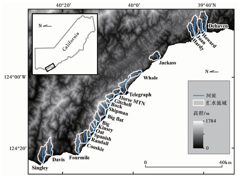	Figure Option View Download New Window
	图 1 美国加利福尼亚北部Mendocino Triple Junction(MTJ)地区区域高程数据为1 arcsec SRTM DEM(http: ∥earthexplorer.usgs.gov/); 河流分布来源于Snyder et al., 2000Fig. 1 The Mendocino Triple Junction(MTJ)region in northern California, USA.

4.1 应用积分法计算河道参数

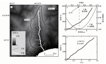
以MTJ区域北部的Davis流域(图2a)为例, 说明如何利用积分法计算河道凹度和陡峭系数:

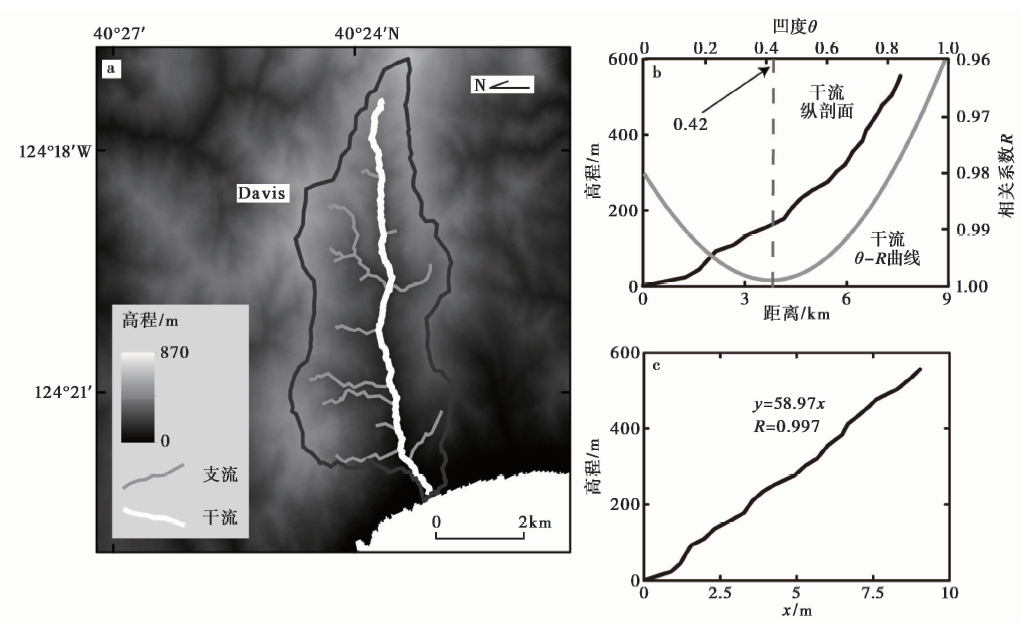	Figure Option View Download New Window
	图 2 Davis流域干流的χ -z变换 a Davis流域范围与干支流分布; b Davis 干流不同凹度下的χ 值与高程的相关系数, 当θ =0.42时, 相关系数最大; c 最佳凹度(0.42)对应的Chi-plotFig. 2 χ -z transformation of the truck river of catchment Davis.

(1)Davis流域的主干道(单一的河道)。本文计算不同凹度下的χ 值及其与高程的相关系数, 发现当θ =0.42时, 相关系数最大, 因此选择0.42作为该流域干流的最佳凹度(图2b)。此时, 河道的Chi-plot如图2c所示。Chi-plot的斜率58.97即主干道的陡峭系数。

(2)多条干流河道, 例如图1中所示的21条流域的主干道。一些学者计算每条主干道的凹度, 然后取其平均值作为参考凹度θ _ref。参考凹度的取值在0.43~0.50之间(Snyder et al., 2000; Perron et al., 2013; Wang et al., 2017)。以θ _ref计算每条干流的Chi-plot, 斜率就是各自的归一化陡峭系数。

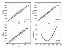
(3)Davis流域, 其中包含1条主干道和多条支流。本文利用式(6)计算了不同凹度值下Davis流域干、支流Chi-plot的高程偏差, 发现当θ =0.45时, 偏差最小(图3)。因此, 0.45可以作为Davis全流域的参考凹度值。

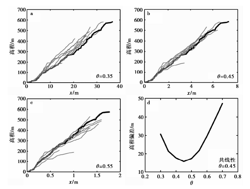	Figure Option View Download New Window
	图 3 Davis流域干支流Chi-plot a— c 凹度值分别为0.35、 0.45和0.55条件下的干支流的Chi-plot; d 不同凹度值下流域Chi-plot的高程偏差, 当θ =0.45时, 偏差最小Fig. 3 Chi-plot of stem and tributaries of catchment Davis.

4.2 陡峭系数与SL、 HI指数的联系

式(9)说明了SL指数与陡峭系数之间确实存在正相关, 但也指出了SL指数有意义的前提是hm/n ≈ 1。因为只有在这种条件下, 河道坡度与距离的倒数之间才存在线性关系。

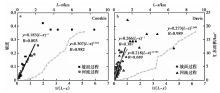
以MTJ区域北部的Cooskie流域干流为例, 本文对河道坡度与河流长度的倒数进行线性回归。如图4a所示, 二者表现出高度的线性相关性(R=0.803)。需要指出的是, 本文对相关关系强弱的判别, 采用Champagnac等(2012)的方法: 高度相关(high correlation), |R|> 0.7; 存在相关性(fair correlation), 0.5< |R|< 0.7; 弱相关(weak correlation), 0.3< |R|< 0.5; 不相关(no correlation), |R|< 0.3。Cooskie河流的凹度θ =0.43(Snyder et al., 2000), 河流长度-汇水面积经验关系式的指数h=2.301(图4a), 则hθ =0.99, 接近于1。这表明Hack提出的SL指数可以用于该流域。

	Figure Option View Download New Window
	图 4 河道坡度、长度和汇水面积之间的关系 a Cooskie, b Davis; 散点图为河道坡度-顺流距离倒数关系图, 灰色虚线为河道顺流距离-汇水面积关系图; L 从河道出水口到分水岭的长度, x 河道溯源距离Fig. 4 Relations between channel slope, stream length and drainage area(a)Cooskie river and (b)Davis river.

对于Davis流域而言, 利用Hack(1957, 1973)的方法计算SL指数则并不合适。如图4b所示, Davis的河道坡度与河流长度的倒数并无显著的线性关系(弱相关, R=0.387)。Davis河流的凹度θ =0.42, 河流长度-汇水面积经验关系式的指数h=2.049, 则hθ =0.86, 不满足式(7)成立的条件。而河道坡度与河流长度的倒数之间存在幂律关系(fair correlation, R=0.689)。实际拟合得到的幂函数的指数(0.725, 图4b)与0.86存在一些误差, 这可能是拟合河流长度-汇水面积经验关系式或者对高程微分等引起的。这也说明了, 为什么一些处于稳态的河流并没有表现出如式(7)所示的线性特征。

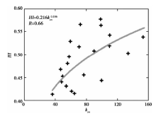
式(14)得到的面积高程曲线积分HI的1个估计量HI^*, 从理论上阐明了HI与陡峭系数k_s之间的正比关系, 为利用流域HI指数表征区域构造活动性强弱提供了理论依据。在实际应用中, 一般都是指定参考凹度计算归一化的陡峭系数(k_sn )。由于选择凹度的不同, k_s和k_sn 之间存在幂律关系(Wobus et al., 2006)。因此, 在理论上, 流域HI和k_sn 两种指数之间也应该存在幂律关系。如图5所示, 本文计算了MTJ区域21条流域的HI和k_sn 指数, 发现两者之间确实存在一定的幂律关系(fair correlation, R=0.662)。

	Figure Option View Download New Window
	图 5 面积高程曲线积分(HI)与河道归一化陡峭系数幂律关系图Fig. 5 Power-law relationship between HI and normalized channel steepness.

4.3 利用χ 值分布判别分水岭迁移方向

如果相邻流域的隆升速率空间均匀, 岩性、气候等条件无显著差异, 同时河道总体落差大致相当, 则可以根据河流源头χ 值分布判别流域边界是否稳定以及分水岭的迁移方向。

位于MTJ区域南部的4条流域(Hardy, Juan, Howard, Dehaven), 基岩隆升速率基本相当, 约0.5mm/a(Snyder et al., 2000)。本文计算这4条流域的χ 值(图6), 发现流域分水岭两侧河段的χ 值大致相当, 因此这些流域的边界基本处于稳定状态。

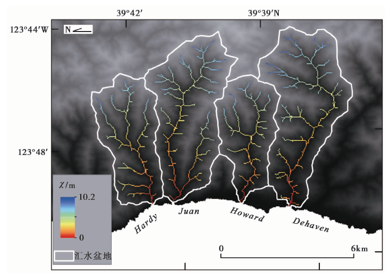	Figure Option View Download New Window
	图 6 稳定的流域Fig. 6 Steady drainage basins.

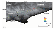
位于MTJ中部的2条流域Telegraph和Whale Gulch, 尽管流域的基岩隆升速率大致相当(1mm/a), 其相邻的流域边界却并不稳定。如图7所示, 分水岭北侧Telegraph的χ 值高于南侧的Whale Gulch流域, 表明分水岭将向北侧移动(图7白色箭头所示)。

	Figure Option View Download New Window
	图 7 不稳定的流域边界箭头(白色、黑色)表示分水岭的迁移方向Fig. 7 Drainage Basins in a state of disequilibrium.

尽管可以用相邻流域河道χ 值的高低判别分水岭的迁移方向, 但这种方法的前提条件是比较严格的: 区域隆升速率无显著差异, 岩性和气候条件大致相当。如图7所示, 相邻的2个流域Horse MTN和Telegraph规模小(流域面积6~8km²), 气候和岩性无显著差异(Merritts et al., 1989; Snyder et al., 2000), 分水岭两侧的χ 值大致相当, 据此而言这2条流域的边界可能是稳定的。然而, 区域地质研究结果表明Horse MTN流域基岩隆升速率为2.3mm/a, 远高于Telegraph流域(1mm/a)(Merritts et al., 1989; Snyder et al., 2000)。理论研究和数值模拟均表明, 在气候和岩性相似的情况下, 分水岭向隆升速率高的一侧移动(Willett, 1999; Willett et al., 2014)。虽然并无直接证据表明, 这2条流域的分水岭向北侧移动(图7黑色箭头所示)。但是, 这至少说明, 在利用χ 值判别分水岭迁移方向的时候, 需要注意该方法适用的前提条件。

5 结论

稳态河道高程剖面分析方法有坡度-面积分析法和积分法2种。前者因计算坡度, 需要对高程数据进行平滑、重采样和微分等一系列操作, 这样会增加计算结果的误差。积分法通过直接求解稳态的河水动力侵蚀方程, 将河道高程以1个积分函数表示出来, 避免了因计算坡度带来的缺点, 确保可以得到高精度的陡峭系数。积分法在理论研究和实际应用中都具有重要价值。在理论上, 积分法用连续函数表达基岩河道, 可以将陡峭系数和一些地貌参数(SL指数、面积高程曲线积分HI)联系起来, 为用这些参数表示区域构造活动信息提供理论支持; 在实际应用中, 该方法不仅可以得到高精度的河道陡峭系数、保持流域干支流共线性特征, 还可以用于判别分水岭的迁移方向。这些优势使得积分法在分析流域河道特征和进行构造地貌的研究中存在广阔的应用前景。

The authors have declared that no competing interests exist.

参考文献

View Option

[1]	陈杰, Wyrwoll K H, 卢演俦, 等. 2006. 祁连山北缘玉门砾岩的磁性地层年代与褶皱过程[J]. 第四纪研究, 26(1): 20—31. CHEN Jie, Wyrwoll K H, LU Yan-chou, et al. 2006. Magnetochronology of the Yumen conglomerates and multi-pulsed folding and thrusting in the Northern Qilian Shan[J]. Quaternary Sciences, 26(1): 20—31(in Chinese). [本文引用:1]
[2]	褚永彬, 朱利东, 陈伟, 等. 2015. 疏勒河上游河流地貌特征及其演化[J]. 第四纪研究, 35(2): 465—474. CHU Yong-bin, ZHU Li-dong, CHEN Wei, et al. 2015. Geomorphology and evolution of the upper Shule River[J]. Quaternary Sciences, 35(2): 465—474(in Chinese). [本文引用:1]
[3]	胡小飞, 潘保田, Kirby E, 等. 2010. 河道陡峭指数所反映的祁连山北翼抬升速率的东西差异[J]. 科学通报, 55(23): 2329—2338. HU Xiao-fei, PAN Bao-tian, Kirby E, et al. 2010. Spatial differences in rock uplift rates inferred from channel steepness indices along the northern flank of the Qilian Mountain, northeast Tibetan plateau[J]. Chinese Science Bulletin, 55(27-28): 3205—3214. [本文引用:2]
[4]	胡小飞, 潘保田, 李琼. 2014. 基岩河道水力侵蚀模型原理及其最新研究进展[J]. 兰州大学学报(自然科学版), 50(6): 824—831. HU Xiao-fei, PAN Bao-tian, LI Qiong. 2014. Principles of the stream power erosion model and its latest progress in research[J]. Journal of Lanzhou University(Natural Sciences), 50(6): 824—831(in Chinese). [本文引用:1]
[5]	李小强, 任金卫, 杨攀新, 等. 2015. 六盘山东西两侧第四纪以来构造差异隆升速率递变性[J]. 第四纪研究, 35(2): 445—452. LI Xiao-qiang, REN Jin-wei, YANG Pan-xin, et al. 2015. Regularity of tectonic differential uplifting rates of both the east and west sides of Liupanshan Mountain since the Quaternary[J]. Quaternary Sciences, 35(2): 445—452(in Chinese). [本文引用:1]
[6]	王一舟, 张会平, 俞晶星, 等. 2013. 祁连山洪水坝河流域地貌特征及其构造指示意义[J]. 第四纪研究, 33(4): 737—745. WANG Yi-zhou, ZHANG Hui-ping, YU Jing-xing, et al. 2013. Geomorphic features of the Hongshuiba river drainage basin in Qilianshan mountain and its insight into tectonic implications[J]. Quaternary Sciences, 33(4): 737—745(in Chinese). [本文引用:1]
[7]	肖萍, 刘静, 王伟, 等. 2015. 青藏高原东南缘芒康地区河流地貌演化的磷灰石U-Th/He记录[J]. 第四纪研究, 35(2): 433—444. XIAO Ping, LIU Jing, WANG Wei, et al. 2015. The evoluiton of fluvial geomorphology of Mangkang area(southeastern Tibetan plateau)recorded by apatite U-Th/He thermochronology[J]. Quaternary Sciences, 35(2): 433—444(in Chinese). [本文引用:1]
[8]	张会平, 张培震, 樊祺诚. 2011. 河流裂点的发育及其溯源迁移: 以鸭绿江-望天鹅火山区为例[J]. 中国科学(D辑), 54(11): 1627—1635. ZHANG Hui-ping, ZHANG Pei-zhen, FAN Qi-cheng. 2011. Initiation and recession of the fluvial knickpoints: A case study from the Yalu River-Wangtian'e volcanic region, northeastern China[J]. Science in China(Ser D), 54(11): 1746—1753. [本文引用:1]
[9]	张会平, 张培震, 吴庆龙, 等. 2008. 循化-贵德地区黄河水系河流纵剖面形态特征及其构造意义[J]. 第四纪研究, 28(2): 299—309. ZHANG Hui-ping, ZHANG Pei-zhen, WU Qing-long, et al. 2008. Characteristics of the Huanghe River longitudinal profiles around Xunhua-Guide area(NE Tibet)and their tectonic significance[J]. Quaternary Sciences, 28(2): 299—309(in Chinese). [本文引用:1]
[10]	Berlin M M, Anderson R S. 2007. Modeling of knickpoint retreat on the Roan Plateau, western Colorado[J]. Journal of Geophysical Research: Earth Surface, 112(F3): F03S06. [本文引用:1]
[11]	Bishop P, Hoey T B, Jansen J D, et al. 2005. Knickpoint recession rate and catchment area: The case of uplifted rivers in Eastern Scotland [J]. Earth Surface Processes and Land forms, 30(6): 767—778. [本文引用:2]
[12]	Champagnac J D, Molnar P, Sue C, et al. 2012. Tectonics, climate, and mountain topography[J]. Journal of Geophysical Research: Solid Earth, 117(B2): B02403. doi: DOI:10.1029/2011JB008348. [本文引用:1]
[13]	DiBiase R A, Whipple K X. 2011. The influence of erosion thresholds and runoff variability on the relationships among topography, climate, and erosion rate[J]. Journal of Geophysical Research: Earth Surface, 116(F4): F04036. doi: DOI:10.1029/2011JF002095. [本文引用:1]
[14]	Duvall A, Kirby E, Burbank D. 2004. Tectonic and lithologic controls on bedrock channel profiles and processes in coastal California[J]. Journal of Geophysical Research: Earth Surface, 109(F3): F03002. doi: DOI:10.1029/2003JF000086. [本文引用:1]
[15]	Duvall A R, Clark M K, Kirby E, et al. 2013. Low-temperature thermochronometry along the Kunlun and Haiyuan Faults, NE Tibetan plateau: Evidence for kinematic change during late-stage orogenesis[J]. Tectonics, 32(5): 1190—1211. [本文引用:1]
[16]	Flint J J. 1974. Stream gradient as a function of order, magnitude, and discharge[J]. Water Resources Research, 10(5): 969—973. [本文引用:2]
[17]	Fox M, Bodin T, Shuster D L. 2015. Abrupt changes in the rate of Andean Plateau uplift from reversible jump Markov Chain Monte Carlo inversion of river profiles[J]. Geomorphology, 238: 1—14. [本文引用:1]
[18]	Fox M, Goren L, May D A, et al. 2014. Inversion of fluvial channels for paleorock uplift rates in Taiwan[J]. Journal of Geophysical Research: Earth Surface, 119(9): 1853—1875. [本文引用:2]
[19]	Gao M, Zeilinger G, Xu X, et al. 2013. DEM and GIS analysis of geomorphic indices for evaluating recent uplift of the northeastern margin of the Tibetan Plateau, China[J]. Geomorphology, 190: 61—72. [本文引用:2]
[20]	Goldrick G, Bishop P. 2007. Regional analysis of bedrock stream long profiles: evaluation of Hack's SL form, and formulation and assessment of an alternative(the DS form)[J]. Earth Surface Processes and Land forms, 32(5): 649—671. [本文引用:1]
[21]	Goren L, Castelltort S, Klinger Y. 2015. Modes and rates of horizontal deformation from rotated river basins: Application to the Dead Sea fault system in Lebanon[J]. Geology, 43(9): 843—846. [本文引用:1]
[22]	Goren L, Fox M, Willett S D. 2014. Tectonics from fluvial topography using formal linear inversion: Theory and applications to the Inyo Mountains, California[J]. Journal of Geophysical Research: Earth Surface, 119(8): 1651—1681. [本文引用:4]
[23]	Hack J T. 1957. Studies of longitudinal stream profiles in Virginia and Maryland [Z]. USGS Professional Paper, 294: 45—97. [本文引用:1]
[24]	Hack J T. 1973. Stream profile analysis and stream-gradient index[J]. Journal of Research of the U. S. Geological Survey, 1(4): 421—429. [本文引用:1]
[25]	Harkins N, Kirby E, Heimsath A, et al. 2007. Transient fluvial incision in the headwaters of the Yellow River, northeastern Tibet, China[J]. Journal of Geophysical Research: Earth Surface, 112(F3): F03S04. doi: DOI:10.1029/2006JF000570. [本文引用:3]
[26]	Holmes A. 1965. Principles of Physical Geology[M]. 2nd ed. Cengage Learning Australia, New York: 20—45. [本文引用:1]
[27]	Howard A D, Dietrich W E, Seidl M A. 1994. Modeling fluvial erosion on regional to continental scales[J]. Journal of Geophysical Research: Solid Earth, 99(B7): 13971—13986. [本文引用:1]
[28]	Howard A D, Kerby G. 1983. Channel changes in badland s[J]. GSA Bulletin, 94(6): 739—752. [本文引用:3]
[29]	Jackson M, Bilham R. 1994. Constraints on Himalayan deformation inferred from vertical velocity fields in Nepal and Tibet[J]. Journal of Geophysical Research: Solid Earth, 99(B7): 13897—13912. [本文引用:1]
[30]	Kerry G, Brown R, Johnson C. 1998. Fission track analysis and its applications to geological problems[J]. Annual Review of Earth and Planetary Sciences, 26(1): 519—572. [本文引用:1]
[31]	Kirby E, Johnson C, Furlong K, et al. 2007. Transient channel incision along Bolinas Ridge, California: Evidence for differential rock uplift adjacent to the San Andreas fault[J]. Journal of Geophysical Research, 112, F03S07. doi: DOI:10.1029/2006JF000559. [本文引用:2]
[32]	Kirby E, Whipple K X. 2001. Quantifying differential rock-uplift rates via stream profile analysis[J]. Geology, 29(5): 415—418. [本文引用:1]
[33]	Kirby E, Whipple K X. 2012. Expression of active tectonics in erosional land scapes[J]. Journal of Structural Geology, 44: 54—75. [本文引用:4]
[34]	Kirby E, Whipple K X, Tang W Q, et al. 2003. Distribution of active rock uplift along the eastern margin of the Tibetan plateau: inferences from bedrock channel longitudinal profiles[J]. Journal of Geophysical Research: Solid Earth, 108(B4): 2217. [本文引用:3]
[35]	Liu D L, Yan M D, Fang X M, et al. 2011. Magnetostratigraphy of sediments from the Yumu Shan, Hexi Corridor and its implications regarding the Late Cenozoic uplift of the NE Tibetan plateau[J]. Quaternary International, 236(1-2): 13—20. [本文引用:1]
[36]	Merritts D, Bull W B. 1989. Interpreting Quaternary uplift rates at the Mendocino triple junction, northern California, from uplifted marine terraces[J]. Geology, 17(11): 1020—1024. [本文引用:2]
[37]	Palumbo L, Hetzel R, Tao M, et al. 2009. Topographic and lithologic control on catchment-wide denudation rates derived from cosmogenic¹⁰Be in two mountain ranges at the margin of NE Tibet[J]. Geomorphology, 117(1-2): 130—142. [本文引用:1]
[38]	Palumbo L, Hetzel R, Tao M X, et al. 2011. Catchment—wide denudation rates at the margin of NE Tibet from in situ-produced cosmogenic¹⁰Be[J]. Terra Nova, 23(1): 42—48. [本文引用:1]
[39]	Pérez-Peña J V, Azañón J M, Azor A. 2009. CalHypso: An ArcGIS extension to calculate hypsometric curves and their statistical moments. Applications to drainage basin analysis in SE Spain[J]. Computers & Geosciences, 35(6): 1214—1223. [本文引用:1]
[40]	Perron J T, Royden L. 2013. An integral approach to bedrock river profile analysis[J]. Earth Surface Process and Land forms, 38(6): 570—576. [本文引用:8]
[41]	Royden L, Perron J T. 2013. Solutions of the stream power equation and application to the evolution of river longitudinal profiles[J]. Journal of Geophysical Research: Earth Surface, 118(2): 497—518. [本文引用:1]
[42]	Royden L H, Clark M K, Whipple K X. 2000. Evolution of river elevation profiles by bedrock incision: analytical solutions for transient river profiles related to changing uplift and precipitation rates [Z]. Transactions of the American Geophysical Union81: Fall Meeting Supplement, Abstract T62F—09. [本文引用:3]
[43]	Rudge J F, Roberts G G, White N J, et al. 2015. Uplift histories of Africa and Australia from linear inverse modeling of drainage inventories[J]. Journal of Geophysical Research: Earth Surface, 120(5): 894—914. [本文引用:1]
[44]	Seeber L, Gornitz V. 1983. River profiles along the Himalayan Arc as indicators of active tectonics[J]. Tectonophysics, 92(4): 335—367. [本文引用:1]
[45]	Snyder N P, Whipple K X, Tucker G E, et al. 2000. Land scape response to tectonic forcing: Digital elevation model analysis of stream profiles in the Mendocino triple junction region, northern California[J]. Geological Society of America Bulletin, 112(8): 1250—1263. [本文引用:9]
[46]	Snyder N P, Whipple K X, Tucker G E, et al. 2003. Channel response to tectonic forcing: field analysis of stream morphology and hydrology in the Mendocino triple junction region, northern California[J]. Geomorphology, 53: 97—127. [本文引用:2]
[47]	Strahler A N. 1952. Hypsometric(area-altitude)analysis of erosional topography[J]. Geological Society of America Bulletin, 63(11): 1117—1142. [本文引用:2]
[48]	Tarboton D G, Bras R L, Rodriguez-Iturbe I. 1989. Scaling and elevation in river networks[J]. Water Resources Research, 25(9): 2037—2051. [本文引用:1]
[49]	Wang W T, Zhang P Z, Liu C C, et al. 2016. Pulsed growth of the West Qinling at~30Ma in northeastern Tibet: Evidence from Lanzhou Basin magnetostratigraphy and provenance[J]. Journal of Geophysical Research: Solid Earth, 121(11): 7754—7774. [本文引用:1]
[50]	Wang Y Z, Zhang H P, Zheng D W, et al. 2014. Controls on decadal erosion rates in Qilian Shan: Re-evaluation and new insights into land scape evolution in north-east Tibet[J]. Geomorphology, 223: 117—128. [本文引用:1]
[51]	Wang Y Z, Zhang H P, Zheng D W, et al. 2017. Coupling slope-area analysis, integral approach and statistic tests to steady-state bedrock river profile analysis[J]. Earth Surface Dynamics, 5(1): 145—160. [本文引用:7]
[52]	Whipple K X. 2004. Bedrock rivers and the geomorphology of active orogens[J]. Annual Review of Earth and Planetary Sciences, 32(1): 151—185. [本文引用:1]
[53]	Whipple K X, Hancock G S, Anderson R S. 2000. River incision into bedrock: Mechanics and relative efficacy of plucking, abrasion, and cavitation[J]. GSA Bulletin, 112(3): 490—503. [本文引用:1]
[54]	Whipple K X, Tucker G E. 1999. Dynamics of the stream-power river incision model: Implications for height limits of mountain ranges, land scape response timescales, and research needs[J]. Journal of Geophysical Research: Solid Earth, 104(17): 17661—17674. [本文引用:1]
[55]	Willett S D. 1999. Orogeny and orography: The effects of erosion on the structure of mountain belts[J]. Journal of Geophysical Research: Solid Earth, 104(B12): 28957—28981. [本文引用:2]
[56]	Willett S D, McCoy S W, Perron J T, et al. 2014. Dynamic reorganization of river basins[J]. Science, 342(6175): 1248765. [本文引用:5]
[57]	Wobus C, Whipple K X, Kirby E, et al. 2006. Tectonics from topography: procedures, promise, and pitfalls[J]. Geological Society of America Special Paper, 398(12): 55—74. [本文引用:6]
[58]	Yang R, Willett S D, Goren L. 2015. In situ low-relief land scape formation as a result of river network disruption[J]. Nature, 520: 526—529. [本文引用:2]
[59]	Zhang H P, Kirby E, Pitlick J, et al. 2017. Characterizing the transient geomorphic response to base-level fall in the northeastern Tibetan plateau[J]. Journal of Geophysical Research: Earth Surface, 122(2): 546—572. [本文引用:2]
[60]	Zheng D W, Clark M K, Zhang P Z, et al. 2010. Erosion, fault initiation and topographic growth of the North Qilian Shan(northern Tibetan plateau)[J]. Geosphere, 6(6): 937—941. [本文引用:1]
[61]	Zheng D W, Zhang P Z, Wan J L, et al. 2006. Rapid exhumation at~8Ma on the Liupan Shan thrust fault from apatite fission-track thermochronology: Implications for growth of the northeastern Tibetan plateau margin[J]. Earth and Planetary Science Letters, 248(1-2): 198—208. [本文引用:1]

2006

0.0

陈杰, Wyrwoll K

, 卢演俦, 等. 2006. 祁连山北缘玉门砾岩的磁性地层年代与褶皱过程[J]. 第四纪研究, 26(1): 20—31.

CHEN

Jie

, Wyrwoll K

, LU

Yan-chou

, et al. 2006. Magnetochronology of the Yumen conglomerates and multi-pulsed folding and thrusting in the Northern Qilian Shan[J]. Quaternary Sciences, 26(1): 20—31(in Chinese).

Nearly continuous exposure of deformed Plio-Pleistocene sediments reveal that the Laojunmiao fold-and-thrust belt is particularly favorable for determining the geometry, style, timing, and rate of active faulting and folding within a foreland basin along the northern margin of the Qilianshan. Paleomagnetic investigations of two Plio-Pleistocene terrestrial successions provide detailed magnetostratigraphy for the Upper Cenozoic strata in this region. Results show that the conglomeratic Yumen Formation is diachronous with the basal age ranging from ca.4Ma in the Niugetao section to ca.3.55Ma in the Qingcaowan west section ca.14km to the northwest on the northeast limb of the anticline. Northwestward lateral propagation and growth of the Laojunmiao fold-and-thrust belt initiated at ca.3Ma in the Niugetao, and ca.1.2Ma in the Qingcaowan west with a rate of ca. 7.8km/Ma. The cross section in the Niugetao provides a conservative estimate of shortening rate of 1.2mm/a and uplift rate of 1.1mm/a since ca. 3Ma. Detailed mapping of the rotational offlap onlap geometrical growth strata at the forelimb indicates multi-pulsed folding and thrusting, which suggests that the Laojunmiao fold-and-thrust belt developed as a result of northeastward migration and propagation of thrusting and folding of the northeastern edge of the Qinghai-Tibetan Plateau.

在我国西部致使玉门砾岩强烈褶皱变形的构造运动是喜马拉雅运动中重要的一幕。祁连山北缘老君庙逆断裂-褶皱带前翼发育的生长地层为认识玉门砾岩褶皱的过程提供了重要证据。通过对这套生长地层及其内部渐进不整合几何形态和结构的详细填图以及磁性地层年代学研究,认为玉门砾岩的底界具有穿时性,其年龄可能由东南向西北变小,其底界年龄在牛胳套剖面约4Ma,在青草湾西剖面约3.55Ma。玉门砾岩的褶皱变形在牛胳套剖面起始于约3Ma,沉积速率由约260m/Ma变为170m/Ma,在青草湾西剖面起始于约1.2Ma。结合构造变形的样式、强度及侵蚀程度推断老君庙逆断裂-褶皱带是以约7.8km/Ma的速率由东南向西北侧向扩展生长的。发育在背斜前翼的多个退覆-超覆生长楔表明玉门砾岩的褶皱变形由3~4个活跃期和平静期组成,这反映了祁连山及其北部前陆盆地内褶皱逆冲席体向前陆方向的不断扩展生长过程, 但并不能简单地以此作为整个祁连山或青藏高原多次垂直隆升的证据。

... 在沉积学研究中, 获取不同地层的沉积时间和厚度, 可以计算沉积速率, 进而反映物源区的隆升剥露特征(陈杰等, 2006 ...

2015

0.0

褚永彬, 朱利东, 陈伟, 等. 2015. 疏勒河上游河流地貌特征及其演化[J]. 第四纪研究, 35(2): 465—474.

CHU

Yong-bin

, ZHU

Li-dong

, CHEN

Wei

, et al. 2015. Geomorphology and evolution of the upper Shule River[J]. Quaternary Sciences, 35(2): 465—474(in Chinese).

Shule River originates from the western part of the Qilianshan Mountain, between Shulenanshan Mountain and Tuolainanshan Mountain. The upper Shule River is located in the Middle Qilian block, differentially controlled by the Northern Middle Qilian Fault Zone and the Southern Middle Qilian Fault Zone. Its landform is the result of the uplift of the Qinghai-Tibetan Plateau. Altyn Tagh Fault, Hanxia-Dahuanggou Fault, Changma Fault, Northern Daxueshan Fault, Tuolainanshan Fault and Shulenanshan Fault are mainly active faults. In the study area, Cenozoic strata spreads in Shule River basin, Changma basin and both sides of the river. Proterozoic strata and Paleozoic strata spread in the middle part of the upper Shule River and mountains surrounding Changma basin. In this study, the ASTER GDEM V002, spatial resolution of 30m, was utilized as basic data, and the hydrology tools were applied in ArcGIS to extract the river profile, Hack profile, SL index, and HI from the upstream basin of the Shule River to analyze fluvial geomorphology, and extract watershed boundary elevation profile to analyze geomorphic evidence left from the basin evolution. There are three obvious fluvial elbows. In each bend of the river, there was a knickpoint and abnormally SL value. SL presents per 100km sectional characteristics. There are abnormal high values or abnormal low value in each section. The river segments with abnormally high SL values, mainly represented faults activity of study area. The obviously highest SL values appear in Tuolainanshan Fault. The linear function was the best fit-function for the river longitudinal profile of the upper Shule River, which indicated that the evolution process of the upper river was in an early stage. The morphology of Hack profiles was convex, which showed that the main factor causing the landform was tectonic uplifting in the upper Shule River. The HI of the Shule River upstream watershed was 0.49. From its river source to 80km afar, the HI was 0.23, which indicated that the stages of river development were different. The distribution interval of the both river sides' HI was 0.292 to 0.547. The HI showed that secondary basins of the river varying in developmental stages from old stage to middle stage to juvenile stage corresponding to the position from source to alluvial fan. The elevation of basin boundary indicated pass gaps position. Fluvial elbows, SL and knickpoints in the river were found close to one another and also near the pass gaps what were distinguished from watershed boundary elevation profile. These geomorphic information allows us to infer that the fluvial reorganization occurred by means of three fluvial captures. The recombinant of ancient Shule River, Changma River and Yema River shaped the current Shule River basin.

疏勒河上游位于中祁连地块,受到中祁连南缘断裂带、中祁连北缘断裂带的差异控制,其地貌是青藏高原隆升的结果.本文以疏勒河上游为研究对象,应用ArcGIS水文分析工具,提取河流纵剖面、Hack剖面、SL参数以及HI,分析了河流的形态特征; 提取流域边界高程剖面,分析了流域演化遗留的地貌证据.研究结果表明,疏勒河上游河流纵剖面以线性函数为最佳拟合函数,说明疏勒河上游河段整体上处于河流发育早期阶段; Hack剖面呈明显的凸形,说明第四纪以来流域所在地区处于强烈的构造抬升; 河流流向转折、SL异常值以及河流纵剖面裂点具有良好的一致性,从流域边界剖面识别的垭口又与上述三者具有对应关系.综合上述河流特征及流域边界剖面所反映的信息,推测研究区发生过3次袭夺事件.古疏勒河、古昌马河以及古野马河的重组塑造了现在的疏勒河流域.

... 褚永彬等, 2015) ...

2010

0.0

胡小飞, 潘保田, Kirby

, 等. 2010. 河道陡峭指数所反映的祁连山北翼抬升速率的东西差异[J]. 科学通报, 55(23): 2329—2338.

Xiao-fei

, PAN

Bao-tian

, Kirby

, et al. 2010. Spatial differences in rock uplift rates inferred from channel steepness indices along the northern flank of the Qilian Mountain, northeast Tibetan plateau[J]. Chinese Science Bulletin, 55(27-28): 3205—3214.

... 胡小飞等, 2010 ...

... 胡小飞等, 2010, 2014 ...

2014

0.0

胡小飞, 潘保田, 李琼. 2014. 基岩河道水力侵蚀模型原理及其最新研究进展[J]. 兰州大学学报(自然科学版), 50(6): 824—831.

Xiao-fei

, PAN

Bao-tian

, LI

Qiong

. 2014. Principles of the stream power erosion model and its latest progress in research[J]. Journal of Lanzhou University(Natural Sciences), 50(6): 824—831(in Chinese).

基岩河道水力侵蚀模型是最近20年发展起来的一项地貌演化定量分析的研究方法.模型基于河流侵蚀基本物理过程、实验观测及经验公式,推导出可以应用的数学模型对河流侵蚀过程进行模拟与构造分析.目前,其主要应用在构造抬升速率研究与地貌演化模拟研究中,但由于模型在简化过程中存在一系列假设,应用中具有一定的不确定性,其中主要的不确定性来自于坡度指数、河道宽度、岩性与沉积物影响等方面,对这些关键参数与问题的定量获取研究也是目前与将来主要的研究热点.在应用基岩河道水力侵蚀模型对地貌分析中,一定要注意其限定因素与不确定因素,否则会不同程度地降低研究结果的可信性.

... 胡小飞等, 2010, 2014 ...

2015

0.0

李小强, 任金卫, 杨攀新, 等. 2015. 六盘山东西两侧第四纪以来构造差异隆升速率递变性[J]. 第四纪研究, 35(2): 445—452.

Xiao-qiang

, REN

Jin-wei

, YANG

Pan-xin

, et al. 2015. Regularity of tectonic differential uplifting rates of both the east and west sides of Liupanshan Mountain since the Quaternary[J]. Quaternary Sciences, 35(2): 445—452(in Chinese).

As a kind of new sedimentary geomorphology since the Quaternary, river terraces are playing an important role in the study of regional tectonic uplift and fault activity. In this article, we collected the previous study achievements of the Yellow River terraces of the east and west Liupanshan Mountain, the Weihe River terrace and the Jinghe River terrace, meanwhile, we incorporated the formation age according to the paleomagnetic and 14 C methods, the measurements of tug-of-war and so on. Based on these data, we built a tectonic differential uplifting rate ( Δ U T ) model to reflect the regional activity and the intensity of tectonic uplift based on the parameters of terraces in both the east and west sides of Liupanshan Mountain. First of all, we compared the tectonic differential uplifting rates of the Jinghe River with the Lanzhou segment of the Yellow River terraces, the results show that there are four times of Δ U T , which are 76.87mm/ka, 42.88mm/ka, 421.06mm/ka and 1050mm/ka. The average of the four rates is 397.70mm/ka. Then, we compared the tectonic differential uplifting rates of the Jinghe River with the Weihe River terraces of Longxi segment, the results show that there are three times of Δ U T , which are 177.37mm/ka, 171.83mm/ka and 168.27mm/ka, and the average rate of them is 172.49mm/ka. Two sets of date in each time have been shown positive. The result implies that the activity of the west Liupanshan Mountain is stronger than the east, meanwhile, the north section of Liupanshan Mountain tectonic belt is more active than the south section and increasing gradually. The primary reason may be the transformation and absorption of the NWW, NNW structural development to the tectonic stress in the west Liupanshan Mountain, while its east side clings to the stable Ordos block and the stress transformation and absorption is not so obvious.

河流阶地作为第四纪以来较新的沉积地貌单元,在研究区域构造隆升和区域断裂活动性方面扮演重要角色.本文利用前人对六盘山东西两侧黄河、渭河及泾河地区阶地研究成果,借用古地磁及 14 C 等方法测定阶地形成年龄和实测阶地拔河高度已有数据,引进构造差异隆升速率( ΔU T )参数来反映区域构造隆升强弱.通过对兰州黄河阶地、陇西渭河阶地与泾河阶地的构造差异隆升速率对比研究表明,第四纪以来,兰州黄河阶地与泾河阶地4个期次平均构造差异隆升速率( Δ U T )分别为76.87mm/ka、42.88mm/ka、421.06mm/ka和1050mm/ka; 平均值为397.70mm/ka; 陇西渭河阶地与泾河阶地3个期次内( Δ U T )分别为177.37mm/ka、171.83mm/ka和168.27mm/ka; 平均值为172.49mm/ka.说明六盘山西侧总体活动性要强于六盘山东侧,同时六盘山构造带北段较南段活动性强,并有逐渐增强趋势.其主要原因可能是六盘山西侧区域系列NWW、NNW活动构造发育对应力的转换和吸收占据重要位置,而六盘山东侧依附于较稳定的鄂尔多斯地块,对区域应力的转换和吸收不明显.

... 李小强等, 2015 ...

2013

0.0

王一舟, 张会平, 俞晶星, 等. 2013. 祁连山洪水坝河流域地貌特征及其构造指示意义[J]. 第四纪研究, 33(4): 737—745.

WANG

Yi-zhou

, ZHANG

Hui-ping

, YU

Jing-xing

, et al. 2013. Geomorphic features of the Hongshuiba river drainage basin in Qilianshan mountain and its insight into tectonic implications[J]. Quaternary Sciences, 33(4): 737—745(in Chinese).

Owing to the intensive uplift of Qilianshan Mountain since Late Cenozoic,the drainage basins that originated the mountain have experienced strong tectonic deformation.So the typical drainage basin characteristics may indicate the tectonic movement of this region.In order to reveal the characteristics of tectonic geomorphology,we carried out our present research on the Hongshuiba River drainage basin,which originates from the interior of the Qilianshan Mountain in the northeastern Tibetan Plateau.Stream networks of Hongshuiba River drainage basin (38°55'~39°30'N,98°10'~98°45'E) were extracted from the DEM data and graded into five levels with Strahler method.Five sub-catchments,Heishui drainage basin,Yanglu drainage basin,Zhangrui drainage basin,Sanchahe drainage basin and upstream region were further chosen for detailed analysis.The bifurcation ratio,basin relief,mean elevation,basin area,stream length,drainage density,and average slope of Hongshuiba drainage basin and the sub-catchments were determined with GIS tools.In addition,we analyzed the slope spectrum of the Hongshuiba drainage basin.Both drainage density and basin area are low,which indicate the drainage network here is still on a primary stage.High bifurcation shows that the drainage basin has experienced intensive tectonic disturbance.From south to north,the bifurcation ratio varies largely.We eliminate the impact of lithology,and regard the difference of bifurcation ratio as an indication of spatial diversity of tectonic movement.In the south part with a high average altitude of 4000m,the bifurcation ratio is 4.08,which reflects less tectonic disturbance.The gentle slope occupies so large area proportion that the slope spectrum shows a bimodal pattern and a peak value is in low slope region.The area with low relief may be regarded as a residual planation surface or the result of fluvial deposition.The middle part may be affected by glacier owing to its high altitude,so the network here were developed not perfectly and the bifurcation ratio may not reflect the tectonic movement.However,the increasing basin relief and the activity of Changma Fault can reflect the increasing impact of tectonic disturbance.In the north part with a high average altitude of 3800m,the basin relief is over 2000m and the bifurcation ratio is above 4.50,both of which indicate that this area has experienced intensive tectonic movement.As a result of the thrust uplift of the east part of Fodongmiao-Hongyazi fault,Hongshuiba River incises terrace deeply near the piedmont outlet.Although the basin relief varies in accord with the tectonic movement,average altitude and slope do not show the same tendency.The increasing average altitude may be resulted from the tectonic background and the slope indicating the local topography steepness may be affected by climate or lithology,both of which require more research.

晚新生代以来,伴随祁连山强烈隆起而塑造的水系流域地貌,其典型特征指示了该区域的最新构造活动。以发源于祁连山中部的洪水坝河为研究对象,利用GIS空间分析工具,提取了整体流域与5个亚流域的河网分支比、地势起伏、平均高程等地貌参数,并对整个流域地形做坡谱分析,获得了洪水坝河水系流域地貌特征。研究表明,洪水坝河流域整体地形起伏大、坡度陡、水系发育程度低,并且流域内部从南向北,河网分支比和地势起伏显著增大。在分析地层岩性和冰川作用等相关因素的基础上,认为这种变化表明流域所受构造活动的影响从南向北显著增强:南部受构造活动的影响微弱,地势平坦,可能是残存的古侵蚀面,亦或是受山间盆地的沉积作用影响; 中部区域由于被昌马断裂东段切穿,断裂带附近区域较弱的抗侵蚀能力与河流的快速下切共同造成了地势起伏的增加; 北部区域受佛洞庙-红崖子断裂西段逆冲活动的影响,坡度及地势起伏大幅增加,表现为地势起伏骤增和强烈的河流下切等地貌特征。上述地貌分析研究,为认识和理解祁连山造山带地貌演化以及控制因素提供了基础数据和思路。

... 王一舟等, 2013 ...

2015

0.0

肖萍, 刘静, 王伟, 等. 2015. 青藏高原东南缘芒康地区河流地貌演化的磷灰石U-Th/He记录[J]. 第四纪研究, 35(2): 433—444.

XIAO

Ping

, LIU

Jing

, WANG

Wei

, et al. 2015. The evoluiton of fluvial geomorphology of Mangkang area(southeastern Tibetan plateau)recorded by apatite U-Th/He thermochronology[J]. Quaternary Sciences, 35(2): 433—444(in Chinese).

The southeastern margin of Tibetan Plateau(TP)is characterized by long-wavelength, low-gradient topography with three nearly parallel largest rivers(Salween River, Mekong River, and Jinsha River)in Asian flowing out of the high plateau across this region. The formation mechanism and evolution process for the large scale landscape and drainage of the SE marginal TP remains elusive. Distributed in the tributary of Mekong upstream(29.56°~29.72°N and 98.01°~98.20°E), 5 samples are collected from Dongdashan pluton in Mangkang-Zuogong region for apatite U-Th/He dating in this study. Our new data shows that the study area experienced a cooling event at the time span 23~15Ma, with the cooling rate dropped from 40℃/Ma to 28℃/Ma or even lower in 5Ma, which is similar to the inversion modeling results. Moreover, most ages concentrate at around 18Ma except the sample TL09-12 which is older than 20Ma, and the age-elevation relationship plot exhibits less obvious correlation. Available low temperature thermochronology data in this region and adjacent area indicate that: the timing, for the formation of high elevation, low relief landscape of southeast and east Tibetan Plateau, is diachronity. So, it is unsuitable for discussing and calculating the regional initial uplift as one unit; the landscape of three river regions is a non-steady transitional one, and the difference of exhumation rates suggests the geomorphic evolution of the Mekong watershed is in the period of unsteady. Furthermore, river erosion plays a dominant role in shaping landscape of this region:(1)The erosion rate in the trunk is much higher than tributary;(2)The high erosion rate and topographic relief is consistence with intensive river incision; and (3)The weak topographic relief is determined by the relative low erosion rate.

青藏高原东南缘地处印度与欧亚板块碰撞侧向逃逸的特殊构造部位,地势起伏相对较缓,形成三江并流的独特地貌格局.然而,对于东南缘大尺度地形地貌形成机制与水系演化的认识仍存在很大的分歧.本文获得的澜沧江流域芒康地区5个基岩样品磷灰石U-Th/He年龄表明该地区在早-中中新世(23~15Ma)经历了一次区域性冷却事件,且冷却速率在5Ma期间从40℃/Ma降低到28℃/Ma以下.目前可获得的青藏高原东缘-东南缘的低温年代学数据表明: 尽管川西-藏东-滇北一带具有相似地貌特征,但高海拔、低起伏地貌面的形成是穿时性的,不能将它作为一个区域上连续的等时面来计算和探讨一个统一的区域抬升启动时间; 三江地区地形属于非稳态的过渡型地形,尤其芒康-左贡地区剥蚀速率的差异比较清晰地展示了澜沧江流域地形演化处于非稳态期.此外,河流下切是塑造澜沧江流域的地形地貌主要驱动力之一: 干流的侵蚀速率远远高于支流的侵蚀速率; 河流下切强烈的地区(如德钦)对应的侵蚀速率及地形起伏度都较大,芒康地区微弱的地形起伏度取决于较低的侵蚀速率.第三纪以来的印度-欧亚板块碰撞导致青藏高原崛起的同时,也对周边尤其藏东南三江地区的地形地貌塑造及气候变化产生重大的影响.

... 肖萍等, 2015 ...

2011

0.0

张会平, 张培震, 樊祺诚. 2011. 河流裂点的发育及其溯源迁移: 以鸭绿江-望天鹅火山区为例[J]. 中国科学(D辑), 54(11): 1627—1635.

ZHANG

Hui-ping

, ZHANG

Pei-zhen

, FAN

Qi-cheng

. 2011. Initiation and recession of the fluvial knickpoints: A case study from the Yalu River-Wangtian'e volcanic region, northeastern China[J]. Science in China(Ser D), 54(11): 1746—1753.

利用数字高程模型(Digital Elevation Model)和数值模拟方法,系统地研究中国东北部鸭绿江上游-望天鹅火山区河流裂点的空间分布特征,构建了裂点溯源迁移模型(Knickpoint Celerity Model),定量地计算裂点溯源迁移速率与流域面积之间的关系.研究结果表明,裂点溯源迁移模型中侵蚀系数K为1.32×10-8,而流域面积指数m为0.69;模拟裂点与实际裂点分布的误差分析表明,二者之间具有较好的一致性;研究区各水系内部裂点的起始溯源迁移速度主要为1～10 mm/a,现今的迁移速率主体为1～6 mm/a.研究结果与日本阿苏火山(Aso Volcano)和房总半岛(Boso Peninsula)火山具有可对比性.本研究为今后深入研究鸭绿江-望天鹅火山区的地貌演化过程提供了基础数据.

... 张会平等, 2008, 2011 ...

2008

0.0

张会平, 张培震, 吴庆龙, 等. 2008. 循化-贵德地区黄河水系河流纵剖面形态特征及其构造意义[J]. 第四纪研究, 28(2): 299—309.

ZHANG

Hui-ping

, ZHANG

Pei-zhen

, WU

Qing-long

, et al. 2008. Characteristics of the Huanghe River longitudinal profiles around Xunhua-Guide area(NE Tibet)and their tectonic significance[J]. Quaternary Sciences, 28(2): 299—309(in Chinese).

Xunhua-Guide area is a part of Late Cenozoic tectonic orogenic systerm along the northeastern Tibetan Plateau.The section of the Huanghe River in this area provides an ideal site to unravel the process of the plateau uplift and incision of the Huanghe River.Although some terrace studies within this region have shown a coupling pattern between the plateau uplift and Huanghe River incision,more analysises are still needed to test the impact of the ongoing uplift on river evolution.It is known that longitudinal profile can be well adjusted to respond the vertical differential uplift and lithological change along a river thus in this paper we have carried out a study on longitudinal profile of the Huanghe River and its 38 tributaries.By utilizing the digital elevation model database,longitudinal profiles along the Huanghe River around Xunhua-Guide area were extracted and analyzed.Our study indicates that 65.8%（25/38）of the longitudinal profiles are convex up,while 34.2%（13/38）show concave features.Determination of the knickpoint location along the profile indicates that 64.0%（16/25）of the 25 convex profiles have their knickpoints near the basin boundary or the contact between basin and range systerm.On the basis of the stream-power incision model,the tectonic expression on the profile is determined.Our logrithmic slope-area plots for the Huanghe River drainage declare that 68.4%（26/38）are upward-convex and the left are almost near the linear state.Consequent analysis reveals that the upward-convex features of the profiles and slope-area plots can be explained by the elevation of the bedrock profile getting higher and higher and the uplift being beyond the incision around the target area.Additionally,we know that in the areas where the rivers run across the pre-Cenozoic high resistant bedrocks,the longitudinal profiles also show a similar upward-convex feature,which indicates that the differential lithology distribution is also another control of the profile feature.In a general view,the longitudinal profiles of the Huanghe River tributaries are well controlled by the Late Cenozoic tectonics and lithological difference,which indicates that the landscape around Xunhua-Guide area is in the pre-steady state or near to the steady state.Meanwhile,our analysis also agrees,to some degree,that the northeastern Tibetan Plateau is one of the newly uplifted parts in the whole plateau frame.

青藏高原东北缘循化-贵德地区晚新生代构造活动强烈,同时晚新生代黄河的发育和演化也提供了研究高原构造隆升扩展以及黄河侵蚀下切过程的理想场所。黄河水系通过调整河流纵剖面的形态在垂向上响应不同的构造隆升以及河床岩性的变化。利用数字高程模型数据,提取黄河水系河流纵剖面形态,利用基岩河道河流水力侵蚀模型（stream-power incision model）为依托,尝试揭示晚新生代以来强烈构造活动在黄河水系河流纵剖面形态特征上的表现。分析发现,在循化-贵德地区岩性分布均匀的新生代盆地内部,黄河水系纵剖面在河流水力侵蚀模型坡度-面积双对数图解中大部分表现为上凸特征,即基岩河道的河床随时间的变化为正值,指示了基岩的隆升速率大于河流的下切侵蚀速率。在河流流经盆地内部不同岩性地区,特别是前新生界地层区,河流纵剖面也表现为一定的上凸特征,表明了新生界与前新生界地层岩性差异对河流纵剖面的控制作用。综合来看,青藏高原东北缘循化-贵德地区黄河水系河流纵剖面形态特征是晚新生代强烈构造活动和岩性差异共同控制的结果,揭示了循化-贵德地区造山系统地形发育仍然处于前均衡或接近均衡状态,同时也从侧面表明青藏高原东北缘地区是整个高原隆升扩展的最新和最前缘部位的时空格局特征。

... 张会平等, 2008, 2011 ...

2007

0.0

... Berlin et al ...

2005

0.0

... Bishop et al ...

... 然而, 有学者(Bishop et al ...

2012

0.0

2011

0.0

... DiBiase et al ...

2004

0.0

2013

0.0

... Duvall et al ...

1974

0.0

... 20世纪70年代以来, 河水动力侵蚀模型(stream-power river incision model)被提出(Flint, 1974 ...

... 该模型可表示为方程(1)(Flint, 1974 ...

2015

0.0

... , 2014, 2015 ...

2014

0.0

... 但方法(3)并不受河道是否处于稳态的约束, 可以被应用于计算大型的、非稳态流域的参考凹度(Fox et al ...

... 至于如何应用积分法提取河道瞬态信号, 这涉及到非稳态的河水动力侵蚀方程的求解(Fox et al ...

2013

0.0

... Gao et al ...

2007

0.0

... Goldrick et al ...

2015

0.0

... Goren et al ...

2014

0.0

... 计算不同凹度值下的Chi-plot, 如式(6)计算相应的高程偏差(Elevation Scatter, 以MisFit表示), 选择最小偏差对应的凹度作为最佳参考凹度值(Goren et al ...

... Goren et al ...

1957

0.0

... Hack, 1957, 1973 ...

1973

0.0

... Hack, 1957, 1973 ...

2007

0.0

... 在宇宙成因核素年代学领域, 一些学者利用河流沉积物中石英颗粒的¹⁰Be浓度, 结合其生长、衰减模型, 计算流域尺度的剥蚀速率(Harkins et al ...

... Harkins et al ...

... , 2000)或一些论文的章节中(Harkins et al ...

1965

0.0

... Holmes, 1965) ...

1994

0.0

... , 1983,1994 ...

1983

0.0

... Howard, 1983), 为从地形高程数据中定量获取区域隆升或侵蚀信息提供了1种新的途径 ...

... Howard et al ...

... 式(2)就是通常所说的稳态的河水动力侵蚀方程(Howard et al ...

1994

0.0

... Jackson et al ...

1998

0.0

... 传统的热年代学, 如 ⁴⁰Ar/³⁹Ar、裂变径迹(Fission Track)、 (U-Th)/He等, 通过样品高程-年龄图(Elevation-Age Plot)的斜率可以得到岩体的隆升剥露速率, 同时图中的年龄拐点则被用于约束岩体隆升速率发生变化的时间(Kerry et al ...

2007

0.0

... , 2003, 2007 ...

... Kirby et al ...

2001

0.0

... Kirby et al ...

2012

0.0

... , 2001, 2012 ...

... Kirby et al ...

... 1 理论意义在数字高程模型(DEM)出现之前, 计算河流不同河段汇水面积的难度很大, 而获取河流长度、坡度等参数则相对容易(Kirby et al ...

... Kirby et al ...

2003

0.0

... 该模型一经提出, 便被广泛应用(Kirby et al ...

... Kirby et al ...

2011

0.0

... Liu et al ...

1989

0.0

... 如图7所示, 相邻的2个流域Horse MTN和Telegraph规模小(流域面积6~8km²), 气候和岩性无显著差异(Merritts et al ...

... 3mm/a, 远高于Telegraph流域(1mm/a)(Merritts et al ...

2009

0.0

... Palumbo et al ...

2011

0.0

... , 2009, 2011 ...

2009

0.0

... 研究发现, 流域HI指数的大小与该区域构造活动强弱呈正相关(P#cod#x000e9 ...

2013

0.0

... Perron et al ...

... 但是, 由于在计算坡度的过程中, 需要对高程进行平滑、重采样和微分等一系列运算, 这样不仅会造成原数据信息的部分损失, 还极易将高程中所含误差再次引入计算过程中, 从而造成回归分析的相关系数不高、回归结果误差偏大等问题(Perron et al ...

... Perron et al ...

... 值与高程值一一对应(Perron et al ...

... , 2017)、保持干支流共线性特征(Perron et al ...

... 这些新的发现, 给积分法注入新的活力, 因而从这个角度上说, 积分法是一门有广阔发展前景的新方法(Perron et al ...

... Perron et al ...

2013

0.0

... , 2013)、求解非稳态河水动力侵蚀方程(Royden et al ...

2000

0.0

... Royden et al ...

... 针对传统的坡度-面积分析方法的诸多缺点, 一些学者(Royden et al ...

... 因此, 该方法起初并未得到广泛应用, 其优势也鲜为人知, 甚至该方法并未以独立完整的论文形式发表, 而仅仅出现在会议展板(Royden et al ...

2015

0.0

... Rudge et al ...

1983

0.0

... 其中, Strahler(1952)提出的长度-坡度指数(length-gradient index, SL)和Hack(1957)提出的面积高程曲线积分(hypsometric integral, HI)2种地貌指标应用非常广泛(Seeber et al ...

2000

0.0

... 6, 受构造的影响很小, 主要与岩性、气候和侵蚀过程等因素相关(Snyder et al ...

... _ref, reference concavity)来计算河道陡峭系数(Snyder et al ...

... 当汇水面积超过1km²后, 以河水动力侵蚀作用为主(Snyder et al ...

... 因此, 该区域一向被视为研究河流响应构造-气候变化的典型案例(Snyder et al ...

... 50之间(Snyder et al ...

... 43(Snyder et al ...

... 5mm/a(Snyder et al ...

... Snyder et al ...

2003

0.0

... Snyder et al ...

... , 2000, 2003 ...

1952

0.0

... 20世纪50年代, 地貌学家曾利用简单的统计模型, 从高程数据中获取一些地貌参数来试图表示构造活动信息(Strahler, 1952 ...

... 对某一流域, 以任意高程z(x)与高程最大值z_max的比值z(x)/z_max为纵坐标, 高程z(x)以上区域的面积A(x)与流域总面积A_max的比值A(x)/A_max为横坐标, 这样绘制的图称为面积高程曲线(Strahler, 1952) ...

1989

0.0

... 大量研究表明, 陡峭系数的高低可以表征区域构造活动的强弱(Tarboton et al ...

2016

0.0

... Wang et al ...

2014

0.0

... Wang et al ...

2017

0.0

... Wang et al ...

... 随着数值计算的发展和高精度地形数据的出现, 越来越多的研究发现, 积分法在获取高精度的河道陡峭系数(Wang et al ...

... 值之间也具有很高的线性相关性, 得到的陡峭系数具有极小的标准误差(Wang et al ...

... Wang et al ...

2004

0.0

... Whipple, 2004 ...

2000

0.0

... Whipple et al ...

1999

0.0

... Whipple et al ...

1999

0.0

... 分水岭的迁移与水系格局重组在造山带的地形演化过程中是十分普遍的(Willett, 1999 ...

... 理论研究和数值模拟均表明, 在气候和岩性相似的情况下, 分水岭向隆升速率高的一侧移动(Willett, 1999 ...

2014

0.0

... 此外, 该方法还可以用于判别分水岭的迁移方向(Willett et al ...

... Willett et al ...

... 即便流域内的河道处于稳态, 流域分水岭也会发生迁移(Willett et al ...

... Willett等(2014)研究认为, 当相邻流域的基岩隆升速率、岩性和气候条件均无显著差异时, 则可以利用分水岭两侧河流的#cod#x003c7 ...

... Willett et al ...

2006

0.0

... Wobus et al ...

... 由于选择凹度的不同, k_s和k_sn 之间存在幂律关系(Wobus et al ...

2015

0.0

... Yang et al ...

2017

0.0

... Zhang et al ...

2010

0.0

... , 2006, 2010 ...

2006

0.0

... Zheng et al ...