四川长宁<em> M</em><sub>S</sub>6.0地震震源干涉成像定位

引用本文

赵博, 高原, 刘杰, 梁姗姗. 四川长宁 M_S6.0地震震源干涉成像定位 [J]. 地震地质, 2020,42(6): 1474-1491.
ZHAO Bo, GAO Yuan, LIU Jie, LIANG Shan-shan. INTERFEROMETRIC SOURCE IMAGING OF SICHUAN CHANGNING M_S6.0 EARTHQUAKE [J]. SEISMOLOGY AND GEOLOGY, 2020,42(6): 1474-1491. 复制到剪切板

DOI:10.3969/j.issn.0253-4967.2020.06.013
Permissions

《地震地质》编辑部所有

四川长宁 M_S6.0地震震源干涉成像定位

赵博¹⁾, 高原^2)),^*, 刘杰¹⁾, 梁姗姗¹⁾

1)中国地震台网中心, 北京 100045

2)中国地震局地震预测研究所, 北京 100036

*通讯作者: 高原, 男, 1964年生, 博士, 研究员, 主要从事地震各向异性和深部构造研究, E-mail: qzgyseis@163.com。

〔作者简介〕赵博, 男, 1984年生, 2018年于中国地震局地球物理研究所获固体地球物理专业博士学位, 高级工程师, 主要从事地震监测和地震波速度结构等方面工作, E-mail: zhaobo@seis.ac.cn。

收稿日期: 2020-01-20

基金项目: 北京市自然科学基金(8194081)资助

摘要

文中利用干涉成像定位方法对2019年6月17日四川长宁 M_S6.0主震及部分余震进行定位。天然地震波振幅的极性和大小随震源机制和辐射花样的变化而变化, 利用原始波形的特征函数可消除震源在不同方位上远场P波的初动极性和大小的不一致性。文中将干涉成像技术应用于天然地震定位, 通过对干涉波形进行偏移和叠加处理, 分别对震源的水平位置和深度进行偏移成像, 确定了主震及较大余震( M_S≥4.0)的震源位置参数, 其中主震的位置为(28.38°N, 104.88°E), 震源深度为8.0km。此外, 还测试了4种不同的速度模型对定位的影响, 结果显示利用震源干涉成像定位方法获得的结果较为稳定。通过计算台阵、台网的响应函数, 评估了台站分布及特征函数周期长短对定位结果的影响。计算得到的特征函数优势周期约为4s, 该周期的台阵、台网响应函数在水平和垂直方向均显示了较好的收敛性和稳定性。

关键词: 地震干涉; 地震定位; 干涉成像; 偏移叠加; 四川长宁地震

中图分类号:P315.2 文献标志码:A 文章编号:0253-4967(2020)06-1474-18

INTERFEROMETRIC SOURCE IMAGING OF SICHUAN CHANGNING M_S6.0 EARTHQUAKE

ZHAO Bo¹⁾, GAO Yuan²⁾, LIU Jie¹⁾, LIANG Shan-shan¹⁾

1)China Earthquake Networks Center, Beijing 100045, China

2)Institute of Earthquake Forecasting, China Earthquake Administration, Beijing 100036, China

Abstract

Seismic interferometry imaging can accurately determine the source location. The main shock and some aftershocks of Sichuan Changning M_S6.0 earthquake occurring on 17th June, 2019 are located with seismic interferometry imaging in this study. This technique is different from the traditional earthquake location method in that it does not use the phase arrival data in the earthquake catalog. Due to the existence of seismic phase picking errors, the traditional earthquake location method has a basic limitation on the amount of location error reduction. Interferometry imaging method directly applies the waveform records for source location and gets the travel time difference information from cross-correlation calculating, thus, greatly reduces the phase reading error. There are three main processes of interferometric imaging location technique, that is, waveforms cross-correlation of onset phases between station pairs, interferometric waveforms migration, and superposition. However, the complex focal mechanism and radiation pattern of natural earthquakes will cause the polarities of the first arrival phases to be different. When performing superposition processing, the addition of the positive and negative amplitudes will reduce the superimposed energy. By calculating the characteristic functions of the original waveform records, the inconsistency of the polarity of the initial phase caused by the different radiation patterns of the source in different azimuths is eliminated. Since the seismic stations used for location are regional network, the distance between station pairs is relatively close, and waveforms cross-correlation can eliminate some velocity disturbances. Besides, there is a certain coupling between origin time and source location. Therefore, the origin time and source location should be decoupled during locating. The waveform cross-correlation between station pairs can subtract the same origin time, thus, eliminating the location error caused by the disturbance of origin time. In addition, an advantage of the interferometric imaging location method is that it increases the amount of available data. The non-repetitive pairing between stations makes the travel time difference data far more than the direct wave phase data, and these travel time difference data are independent of each other and have no correlation. In this study, the natural earthquakes are located by applying interferometric imaging technology with cross-correlation migration kernel function. After migration and superposition of interferometric waves, the horizontal position and depth of the sources are imaged. The location of the main shock is(28.38°N, 104.88°E, 8.0km), and it is on the west of the aftershock belt. We compared the result from this study with the results of USGS(28.40°N, 104.95°E, 10km), GFZ(28.43°N, 104.94°E, 10km)and CENC(28.34°N, 104.90°E, 16km). The epicenter positions of the four results are relatively consistent, and the deviation is within 0.07°. The depth from our study is consistent with the results from USGS and GFZ, and the difference is 2km. In this study, the depths of M_S4.0~4.9 aftershocks are 5km. Three M_S5.0~5.9 aftershocks are distributed in the depth of 8~10km. The Changning earthquake sequence is located at the western end of the Changning anticline, which is the main geological structure in the Changning area and trending NWW-SEE generally. The anticline is about 100km long from east to west, and about 20km wide from north to south. The Changning anticline was formed in the Mesozoic Era. It was pushed by the NE-SW trending tectonic stress at that time, and accompanied by multiple small faults, shown as high-angle compressive thrust faults. The epicenter distribution shows that the aftershock belt is distributed along the NWW direction. After interferometric imaging location, the average travel time residual is 0.6s. In this study, we used four different velocity models(CodaTomo, Crust1.0, IASPI91 and SIMPLE)for calculating the theory travel time for migration. The effects of four different velocity models on the location are tested and the results show that the seismic interferometric imaging location method is stable. The average travel time residuals of four velocity models are 0.66s, 0.68s, 0.80s, and 0.71s. By calculating the array/network response function, the influence of the station distributions and the length of the characteristic function window on the positioning result are evaluated. The network response functions with four dominant frequencies at 0.01Hz, 0.05Hz, 0.1Hz and 0.25Hz were calculated and compared. The network response functions have fewer local maximums but converge slowly at 0.01Hz, 0.05Hz, and 0.1Hz. In the depth direction, the resolution is very low. The dominant frequency of the eigenfunction calculated in this study is about 0.25s. At this frequency, the network response function shows good convergence and stability in both horizontal location and source depth.

Keyword: seismic interferometry; earthquake location; interferometic imaging; migration and superposition; Sichuan Changning earthquake

文章图片

0 引言

2019年6月17日22时55分, 四川省宜宾市长宁县发生了M_S6.0地震。截至2019年7月8日8时, 中国地震台网共监测并纪录到M_L2.0以上地震232次, 其中5.0~5.9级地震4次, 4.0~4.9级地震6次, 3.0~3.9级地震54次。中国地震台网中心发布的四川长宁主震震中位于(28.34°N, 104.90°E), 震源深度16km, 震级为M_S6.0。

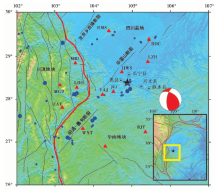
四川地区位于青藏高原东缘, 是中国中强地震的多发区, 2008年汶川M_S8.0地震之后该区发生过2次M_S7.0地震(即芦山地震和九寨沟地震)。前人通过地震序列精定位与震源机制反演、区域速度结构以及大地测量等研究揭示, 印度板块的N向推挤使青藏高原中下地壳的物质向E运移, 在四川盆地周围产生推覆逆冲作用, 导致四川盆地与青藏高原交界地区发生多次较强地震(高原等, 2013, 2018; 张广伟等, 2013; 赵博等, 2013, 2018; 易桂喜等, 2016, 2017; 梁姗姗等, 2018; Jin et al., 2019; 刘小梅等, 2019)。本次四川长宁M_S6.0地震发生在四川盆地东南缘(图 1), 其东南部为华南地块, 西部为川滇地块。该地区位于川南低陡断褶带和川西南低缓断褶带的交切复合部位(朱利峰等, 2016)。长宁地震周边M_S4.0~5.9地震分布较多, 其SW向为昭通-鲁甸断裂, 曾于2014年发生了M_S6.5鲁甸地震。自2018年以来, 长宁地区发生过多次M_S4.0以上地震, 其中离本次地震震中较近的有2018年12月文兴M_S5.7地震和2019年1月珙县M_S5.3地震(图 1)。

Figure Option
View Download New Window

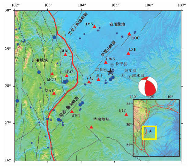图 1 台站与历史地震分布图
红色三角形为台站, 黑色五角星为长宁M_S6.0地震震中, 蓝色大圆点为5.9≥ M_S≥ 5.0的历史地震, 蓝色小圆点为4.9≥ M_S≥ 4.0的历史地震, 沙滩球为主震的震源机制解^①(①www.usgs.gov。), 红色曲线为构造块体边界, 黑色曲线为断层位置, 插图黄色方框为研究区域Fig. 1 Distributions of seismic stations and historical earthquakes.

长宁地区主要的地质构造为长宁背斜, 其总体走向为NWW-SEE, 东起叙永县, 分布于兴文县、长宁县, 西至珙县, EW长约100km, SN宽约20km(蔡一川等, 2015)。长宁背斜形成于中生代, 受当时的NE-SW向构造应力推挤, 生成多个小断裂, 为高角度挤压性逆冲断层。新生代以来, 主压应力场发生了变化。根据该地区历史震源机制解数据反演得到的区域主压应力方向为NWW-SEE(赵博等, 2019), 剪切波分裂研究结合区域应力场分布给出的该地区的主压应力方向为近NW-SE, 但在震中西北的华蓥山断层附近, 剪切波分裂的快波偏振方向呈NE-SW向(石玉涛等, 2013; 高原等, 2018)。长宁背斜现今的构造活动较为平静, 其北侧的基底面深度约为15km。在深部结构背景方面, 最新的研究结果表明, 长宁地震与印度板块在缅甸弧下方深俯冲至地幔转换带并在地幔转换带内形成的 “ 大地幔楔” 结构密切相关, 在该 “ 大地幔楔” 结构中存在板块被拖拽至地幔转换带内, 其内含水沉积层物质脱水或地幔角流引起的热湿物质上涌等动力学过程(Lei et al., 2009, 2016, 2019), 该过程或许对长宁地震的发生具有重要作用。

震源位置参数是确定发震构造的重要依据(易桂喜等, 2015), 也为其他地震学问题研究提供了基础参数。线性和非线性地震定位都需建立地震波走时方程。大部分线性定位以盖格方法(Geiger, 1912)为基础, 建立震源到台站的P波或S波走时方程, 这种单程传播路径上的速度扰动对定位结果有一定的影响。双差定位(Waldhauser et al., 2000)通过求解2个事件到同一台站的到时差以消除路径上的速度扰动, 但该方法属于相对定位, 且受到初始震源深度位置的影响。

近年来, 干涉地震学发展迅速, 基于地震波干涉理论可对震源进行成像(Schuster et al., 2000, 2004)。震源成像在勘探地震领域应用较多, 由于其定位的精确性, 常被用来定位矿塌后失踪的矿工、确定塌陷或爆炸位置及石油勘探中地下的位置信息(Schuster, 2009)。在定位矿塌和被困矿工位置时, 将波形偏移技术应用于震源干涉叠加成像中, 可显著提高定位的精确性和稳定性(Hanafy et al., 2007; Cao et al., 2012)。本研究将地震干涉成像技术应用于天然地震, 对2019年6月17日四川长宁M_S6.0地震及其较大余震进行定位。

1 定位方法与数据处理

1.1 互相关干涉成像定位

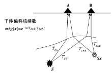
干涉成像定位属于一种非线性能量叠加定位方法。将研究区域网格化, 建立水平和深度方向三维网格, 对每个网格点计算到2个台站的走时差, 作为偏移核函数(Schuster et al., 2004), 将该核函数用于干涉波形的偏移处理, 并对所有偏移后的干涉波形进行叠加。搜索三维网格空间的所有节点(如图 2), 其中真实震源位置的振幅叠加能量最大(Schuster et al., 2000; 赵博等, 2018)。在定位时, 计算空间某点Sx分别到台站A和B的理论走时, 求得2个台站的到时差T_Sx_B-T_Sx_A, 该到时差即为干涉波形的峰值与“ 0时刻” 的理论偏移值。搜索所有网格点, 将所有干涉波形向0时刻偏移并做振幅叠加, 其中叠加能量最大的网格点就是真实的震源位置。该方法利用观测波形直接进行互相关干涉, 其获取的时间信息比震相报告更加精确。同时, 进行互相关干涉可在一定程度上减弱波场在传播过程中的速度扰动。另外, 台站对间的互相关等效于观测震相做差, 可以减去共同的发震时刻因子, 对发震时刻和震源位置进行解耦, 消除发震时刻的不准确性对震源位置的影响。

	Figure Option View Download New Window
	图 2 震源干涉成像(引自赵博等, 2018) 偏移核函数mig(x)=e^-^iω(T_Sx_B-T_Sx_A), S为震源位置, Sx为可能的震源位置, A、 B为地震台站Fig. 2 Interferometric seismic source imaging (after ZHAO Bo et al., 2018).

1.2 波形数据处理

本研究利用震中周围150km内的四川、云南和贵州(SC、 YN和GZ)地震台网的13个固定地震台站的波形数据进行互相关, 计算得到了78条干涉波形, 台站分布见图 1。其中最近的台站为四川台网的汉王山台(SC-HWS), 震中距为36km。截取主震发震时刻开始—震后60s的原始波形记录(图 3), 主要包含P波的波形信息。对主震进行定位时, 通过人工挑选出P波初动明显的波形数据; 对余震进行定位时, 挑选P波初动窗口前、后信噪比> 5的波形数据。对所有波形进行去均值、去线性趋势和振幅归一化处理。

	Figure Option View Download New Window
	图 3 原始波形记录 M_S6.0主震的垂直分量波形记录, 从上到下按震中距排序, 每条波形左侧的字母为台站代码Fig. 3 Original seismic waves records.

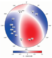
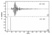
不同于人工爆炸源, 天然地震的震源机制比较复杂, 初动震相的极性和大小随方位角变化很大。我们计算了长宁M_S6.0主震的P波远场辐射花样(图 4)(震源机制解引自www.usgs.gov), 并对台站的位置进行下半球投影, 可以看出P波辐射能量的大小和极性随方位角变化而变化, 这种现象在成像的叠加过程中将直接影响叠加能量的大小。为此, 使用原始波形的归一化特征函数消除初动震相极性及能量的方位差异。本研究利用长短时窗能量比计算原始波形的特征函数(图 5), 并用其进行干涉成像定位。特征函数能够很好地反映初至到时, 并且统一初动方向, 使不同辐射方位的初动极性一致(赵博等, 2018)。

	Figure Option View Download New Window
	图 4 震源P波的远场辐射花样红色表示极性为正, 蓝色表示极性为负; 黑色三角形为台站在下半球投影的位置Fig. 4 P wave radiation patterns of earthquake source.

	Figure Option View Download New Window
	图 5 原始波形与其特征函数 a 原始波形记录; b 特征函数Fig. 5 Original seismic wave and its characteristic function.

2 定位结果与讨论

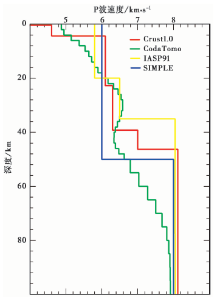
本研究选择了4种速度模型进行成像定位, 如图 6 所示。 CodaTomo模型^① (①赵博, 高原, 2018, 青藏高原东缘地震波速度结构（内部材料）。)是利用尾波干涉速度成像获得的区域P波速度结构; Crust1.0模型(Laske et al., 2013)是全球1°×1°地壳速度模型; IASPI91(Kennett, 1991)是全球大尺度速度模型; SIMPLE模型是本研究设置的一层简单的均匀地壳速度模型, 假定整个地壳厚50km, 速度均匀, 为6.0km/s。

	Figure Option View Download New Window
	图 6 P波速度模型Fig. 6 P wave velocity models.

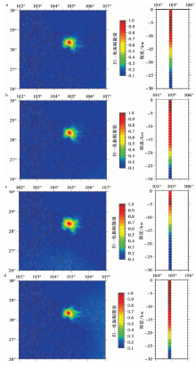
利用上述4种速度模型计算偏移时间, 并对互相关波形进行偏移处理, 如图 7 所示。其中, 图7a为按台站对之间震中距的差值进行排序的干涉波形; 图7b—e分别为利用上述4种速度模型进行偏移后的干涉波形。扣除台站对之间的走时差后, 干涉波形在0时刻附近对齐。将震源区在水平方向进行0.01°×0.01°网格化处理, 深度方向的网格长1km, 对每个节点计算干涉偏移时间, 并对所有干涉波形进行偏移叠加, 振幅能量最大的网格点即为震中位置。图8a—d为利用4种模型得到的震源干涉成像定位结果, 震中位置和深度结果见表1。

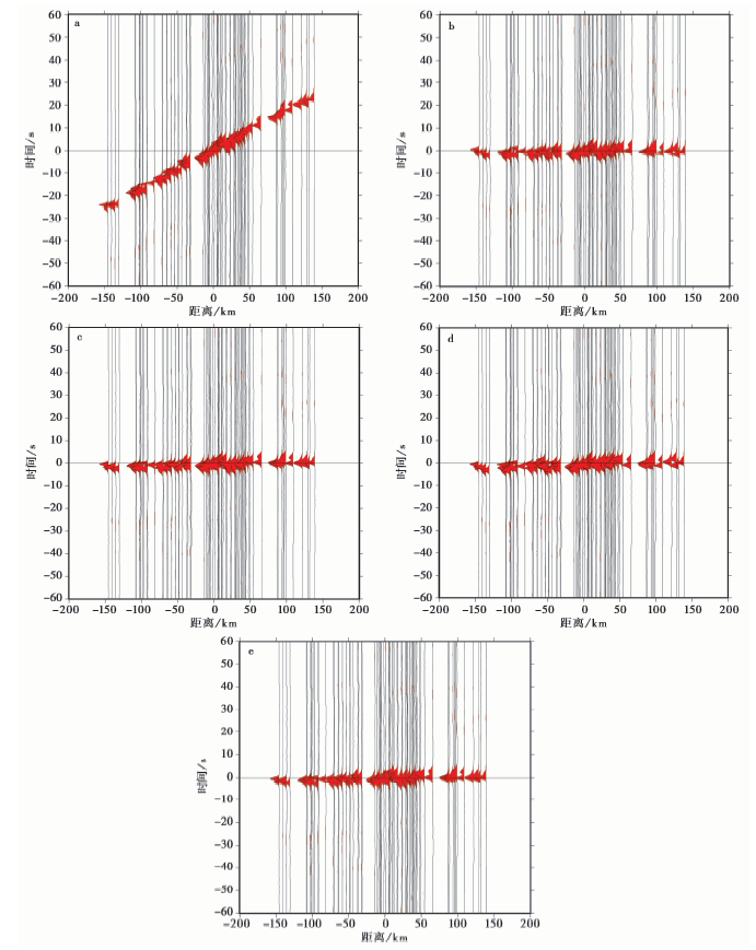	Figure Option View Download New Window
	图 7 干涉波形偏移 a 按震中距差值排序的互相关波形; b—e分别为用图6中的4种速度模型(CodaTomo、 Crust1.0、 IASPI91 和SIMPLE)计算理论偏移时间后的偏移波形Fig. 7 Interferometic waveforms migration.

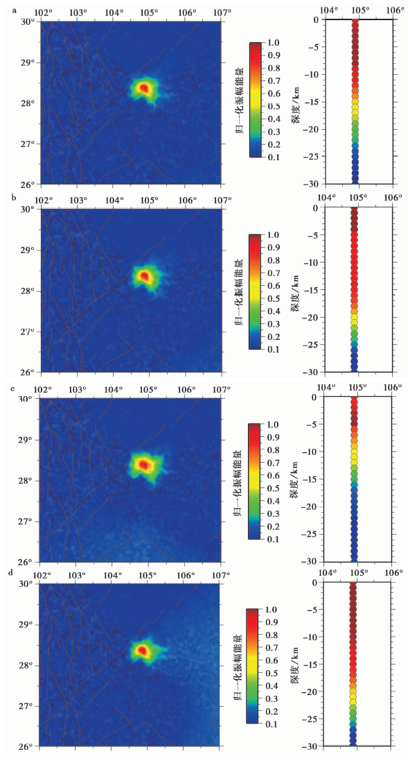	Figure Option View Download New Window
	图 8 震源干涉成像结果 a—d 分别为基于CodaTomo、 Crust1.0、 IASPI91和SIMPLE 4种模型的成像定位结果Fig. 8 The result of interferometic source imaging.

表1 本文的主震定位结果与其他机构的结果对比 Table1 Comparison of the main shock location between the results in this paper and other institutions

4种不同模型的定位结果均相对稳定, 在水平和深度方向变化不大。 CodaTomo模型和Crust1.0模型为区域速度模型, 较为精细, 2种模型定位结果的经、纬度均只差0.01°, 在深度方向二者相差4km。图8a、 8b显示, 在深度方向上, CodaTomo模型的收敛区间为4~9km, 最大偏移叠加能量点位于8km; Crust1.0模型的收敛范围为0~5km, 最大偏移叠加能量点位于4km。 Crust1.0模型在深度方向的分辨率低于CodaTomo模型, 可能是由于后者在浅部更为精细所致。经过对比, SIMPLE模型作为本研究给出的测试模型, 其定位结果也相对可靠, 但图8c显示, 在深度收敛方面, 简单的一层速度对深度的约束有一定缺陷。对比该结果与CodaTomo模型和Crust1.0模型的结果可知, 水平向上的差别在0.02°之内, 深度相差2km。本研究的结果与易桂喜等(2019)的研究结果(表1)也非常接近, 我们利用易桂喜等(2019)使用的1D速度模型进行了干涉成像定位, 得到的结果为(28.40°N, 104.87°E, 5km), 两者在经、纬度和深度方向都比较接近。

干涉成像定位与传统的走时定位相比有其独特的优势:

(1)干涉定位直接利用波形进行成像定位, 避免了拾取初至到时过程中的不准确性引起的误差。

(2)在相同的台网、台阵布局下, 干涉波形的数据量较单台数据量大得多。例如, 理论上具有N个台站的台网, 其干涉波形的数据量为N×(N-1)/2, 即有N×(N-1)/2条干涉波形可用于定位; 而在同样的台网布局下, 直接走时定位的数据量只有N个。

(3)互相关干涉的偏移核函数为同一震源到2个不同台站的走时差, 对于区域地震定位, 可在一定程度上消除射线在传播路径上的速度扰动。上文选择了不同速度模型进行了测试, 在速度模型有变化的情况下, 定位扰动均在可接受的范围内, 其中水平扰动为±0.03°, 深度为±4km。

(4)台站对之间的互相关计算可减去相同的发震时刻, 从而消除因发震时刻不准确引起的位置误差。

(5)利用不同台站对间的走时差定位比传统的单台走时对震源位置的约束要强, 每次迭代的最佳位置需同时使2个台站的走时残差最小。本研究选择了完全偏向震中北侧的4个台站——HMS、 ROC、 LZH和HWS(图 1)进行网外定位测试, 利用干涉成像定位法产生了6条干涉波形, 并进行偏移叠加成像, 得到的震中位置为(28.39°N, 104.92°E, 5km)。而盖格法只能利用4个台站的绝对走时信息进行定位, 得到的结果是(29.13°N, 104.89°E, 7km)。可见, 在同样条件下盖格法的定位误差较大, 其走时残差达17.8s。

本研究对长宁M_S6.0主震、 4个M_S5.0以上地震和6个M_S4.0以上地震进行了震源干涉成像定位, 震源位置见图 9。震中分布显示, 长宁震源区位于长宁背斜的西段。长宁背斜的东段, 即叙永—兴文段的走向为NW-SE, 西段即珙县段为近EW向。本次长宁M_S6.0地震序列发生在长宁背斜的西段, 余震序列自主震向W展布。在地震定位时较难确定震源深度, 而基于不同资料、不同方法得到的震源的含义是有差异的(高原等, 1997)。本研究中利用初动进行定位, 得到的是起始破裂深度。研究结果显示, 主震的震源深度为8km, 5次M_S4.0~4.9余震的震源深度均约为5km。 M_S5.1、 M_S5.6和M_S5.4余震的震源深度分别为8km、 8km和10km, M_S5.3余震的震源深度为4km。剖面AB显示了主震及较大余震的分布情况。长宁余震序列主要沿NWW向分布, 有3次5级以上余震分布在西部, 且震源深度较东部深。易桂喜等(2019)对大量余震做了重新精确定位, 结果表明本次余震序列的深度呈西深东浅的特征。

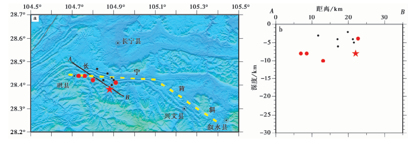	Figure Option View Download New Window
	图 9 主震及余震的震中及深度分布 a 主震与余震震中分布, AB为深度剖面的位置, 黄色虚线为长宁背斜的位置; b AB深度剖面Fig. 9 The distribution of main shock and aftershocks on horizontal and vertical directions.

3 定位精度分析

3.1 干涉波形走时残差

利用不同模型的定位结果计算的每个台站对之间的干涉波形走时残差分布(即理论走时与实际观测走时之差)结果见图 10。

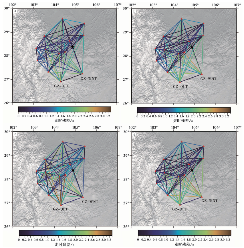	Figure Option View Download New Window
	图 10 走时残差分布 a—d 分别为基于图6中的4种模型CodaTomo、 Crust1.0、 IASPI91和SIMPLE得到的走时残差, 台站对间的直线颜色表示走时残差的大小Fig. 10 Travel time residual distribution.

其中, 基于CodaTomo模型和Crust1.0模型得到的各台站对的平均走时残差分别为0.66s和0.68s, IASPI91模型的平均走时残差为0.80s, SIMPLE模型的平均走时残差为0.71s。图10a和10b所示的整体走时残差水平较低, 与其所使用的2种模型更符合区域实际的速度结构有关。在图9c和9d中, 台网东南缘2个台站GZ-QLT和GZ-WNT的干涉波形走时残差较大, 但这2个台站对于整个台网的布局又非常重要, 使台站方位角能够很好地覆盖, 因此在定位时保留了这2个台站的数据, 并进行干涉定位。

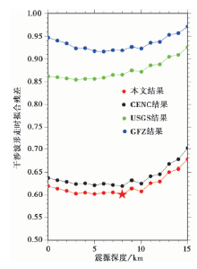
下面将分析本研究的结果与CENC、 USGS和GFZ等给出的结果在深度方向的定位精度。本文定义的干涉波形的走时拟合残差为 $\sum \frac{Δ t_{i, j}}{Δ D_{i, j}},$ 其中, Δ t_i_,_j表示第i、 j个台站对间的干涉波形偏移后与 “ 0时刻” 的偏离时间, Δ D_i_,_j表示第i、 j个台站对间的震源距之差。拟合残差越低, 则表明干涉波形理论偏移时间与实际观测时间越接近。利用前文提到的区域精细速度CodaTomo模型计算了本研究结果与CENC、 USGS和GFZ结果的干涉波形走时拟合残差(图 11)。基于各机构定位结果的水平位置, 在深度方向搜索0~15km之间不同深度的干涉波形理论偏移时间与 “ 0时刻” 的偏差, 并计算走时拟合残差。结果显示, 本研究结果(深度=8km)对应的走时拟合残差最小, 约为0.6s。用CENC的结果进行深度搜索, 在该速度模型下, 走时拟合残差略大于本文的结果。 USGS和GFZ结果的走时拟合残差较大, 这可能与其利用远震数据和大尺度速度模型有关。

	Figure Option View Download New Window
	图 11 干涉波形走时拟合残差五角星表示本研究结果的最优深度位置Fig. 11 Travel time fitting residuals of interferometric waves.

3.2 台阵、台网响应函数

计算台阵响应函数ARF可以得到台阵、台网结构对震源能量中心位置定位的不确定性的影响, 这主要体现在台网布局、台间距以及台网空隙角等的影响(Rost et al., 2002; 王晓欣等, 2017)。

$ARF = {|\frac{1}{N} \overset{N}{\sum_{j = 1}} e^{2 π if Δ t_{j} (x, y, z)}|}^{2}$ (1)

式(1)中, ARF为台阵、台网响应函数, N表示台站数量, f为频率, Δ t_j为震源能量中心周边一点到第j个台站的走时与震源能量中心到第j个台站的走时差。

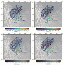
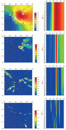
ARF反映了在当前台网布局下, 在优势频率f确定后, 对叠加能量衰减快慢程度和定位结果收敛性的评估。本研究所用特征函数的优势频率约为0.25Hz, 计算得到的0.01Hz、 0.05Hz、 0.1Hz和0.25Hz的台阵响应函数如图 12 所示。在当前定位台站分布下, 不同频率在水平和深度方向的定位收敛程度不同。图12a和12b分别为0.01Hz和0.05Hz频率下的台阵响应函数, 可以看出在水平方向收敛较好, 但收敛较慢, 局部极值较少, 而深度方向的分辨率较差。图12c为0.1Hz频率的台阵响应函数, 其水平方向收敛较快, 局部极大值也很少, 但深度方向的分辨率仍然较低。图12d为0.25Hz频率的台阵响应函数, 该频率是本研究所使用的干涉波形的优势频率, 在水平方向定位收敛很快, 最大能量中心范围迅速收缩。在深度方向的分辨率也较前3个频率有明显提高。

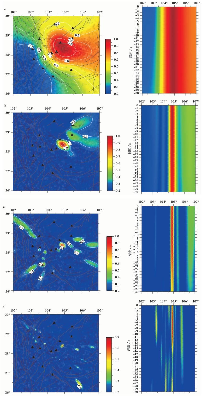	Figure Option View Download New Window
	图 12 台阵响应函数 a—d分别为0.01Hz、 0.05Hz、 0.1Hz和0.25Hz 4个优势频率的台阵响应函数; 左侧为水平方向的台阵响应函数, 右侧为深度方向的台阵响应函数Fig. 12 Array response functions.

4 结论与讨论

天然地震的震源机制具有复杂性, 其辐射花样随方位角的变化而变化, 这使台站记录到的地震波形的初动极性和能量大小随方位而变化, 因此常规的干涉与偏移叠加处理很难用于天然地震波形的定位中。计算天然地震原始波形的特征函数可以很好地统一初动极性与能量大小, 经此处理的天然地震波形即可通过偏移叠加技术进行震源成像定位。对比本研究的结果与易桂喜等(2019)、 CENC、 USGS和GFZ等发表的该次地震的参数信息可知, 地震干涉法在天然地震震源成像、确定震源位置方面是可行的, 其定位结果是可靠的。

互相关型干涉等效于地震波传播路径之差, 相应地, 其偏移核函数也反映了走时差。另外, 干涉处理中的互相关计算避免了人为拾取到时的误差。通过互相关型干涉可在一定程度上消除传播路径上由于速度扰动而引起的位置偏差, 故速度扰动对该方法的影响不大。而台站对之间的波形互相关等效于对初至震相的到时做差, 从而消除了发震时刻的扰动对震源位置的影响。本研究利用4种不同的速度模型进行了震源成像定位, 得到的结果较为一致, 水平向的差别为0.01°~0.02°。 USGS和GFZ等机构利用远场台站及全球大尺度速度模型进行定位, 其发布的位置信息在水平方向较为精确, 而在深度方向上误差较大。在震源深度方面, 在缺少较近台站(震中距≤ 10km的台站)约束的情况下, 本研究利用CodaTomo模型定位的主震震源深度为8km, 与易桂喜等(2019)的研究结果有3km的差别。而利用易桂喜等(2019)研究中用到的速度模型进行干涉成像定位, 得到的震源深度为5km。综上所述, 基于CodaTomo、 Crust1.0、易桂喜等(2019)的模型、 IASPI91以及1D均匀模型, 利用干涉成像定位法得到的震源深度均为4~8km。

台阵、台网响应函数可反映当前台网结构布局对定位精度的影响。本研究所利用的干涉波形的优势频率为0.25Hz, 该频率的台阵响应函数在水平方向收敛最快, 最大叠加能量区域的范围非常小, 表明水平定位精度较好。而深度方向的台阵响应函数的收敛速度相对较慢, 这与无近台参与定位有关。但在现有台网布局下, 我们所用的4s周期的特征函数比其他频率收敛更快。

定位结果显示, 四川长宁M_S6.0地震的主震震源位于(28.38°N, 104.88°E, 8.0km), 主震及余震主要分布在长宁背斜西段, 余震自主震向W展布, 主震及较大余震的震源深度均分布于0~10km。

参考文献

文献列表

[1]	蔡一川, 王宇航. 2015. 四川长宁地区宽频带数字近震记录特征[J]. 四川地震, 154(1): 1—5. CAI Yi-chuan, WANG Yu-hang. 2015. The broadband digitalized recorded characteristic of near earthquakes in Changning area[J]. Earthquake Research in Sichuan, 154(1): 1—5(in Chinese). [本文引用:1]
[2]	高原, 石玉涛, 陈安国. 2018. 青藏东缘地震各向异性、应力及汶川地震影响[J]. 科学通报, 63(19): 1934—1948. GAO Yuan, SHI Yu-tao, CHEN An-guo. 2018. Crustal seismic anisotropy and compressive stress in the eastern margin of the Tibetan plateau and the influence of the M_S8. 0 Wenchuan earthquake[J]. Chinese Science Bulletin, 63(19): 1934—1948(in Chinese). [本文引用:2]
[3]	高原, 王琼, 赵博, 等. 2013. 龙门山断裂带中南段的一个破裂空段: 芦山地震的震后效应[J]. 中国科学(D辑), 43(6): 1038—1046. GAO Yuan, WANG Qiong, ZHAO Bo, et al. 2013. A rupture blank zone in middle south part of Longmenshan Faults: Effect after Lushan M_S7. 0 earthquake of 20 April 2013 in Sichuan, China[J]. Science in China(Ser D), 43(6): 1038—1046(in Chinese). [本文引用:1]
[4]	高原, 周蕙兰, 郑斯华, 等. 1997. 测定震源深度的意义的初步讨论[J]. 中国地震, 13(4): 321—329. GAO Yuan, ZHOU Hui-lan, ZHENG Si-hua, et al. 1997. Preliminary discussion on implication of determination on source depth of earthquake[J]. Earthquake Research in China, 13(4): 321—329(in Chinese). [本文引用:1]
[5]	梁姗姗, 雷建设, 徐志国, 等. 2018. 2017年四川九寨沟 M_S7. 0强震的余震重定位及主震震源机制反演[J]. 地球物理学报, 61(5): 2163—2175. LIANG Shan-shan, LEI Jian-she, XU Zhi-guo, et al. 2018. Relocation of aftershocks of the 2017 Jiuzhaigou, Sichuan, M_S7. 0 earthquake and inversion for focal mechanism of the mainshock[J]. Chinese Journal of Geophysics, 61(5): 2163—2175(in Chinese). [本文引用:1]
[6]	刘小梅, 吴晶, 梁春涛, 等. 2019. 龙门山断裂带最新地震活动特征及其意义[J]. 地球物理学报, 62(4): 1312—1322. LIU Xiao-mei, WU Jing, LIANG Chun-tao, et al. 2019. The latest seismicity characteristics and significance in Longmenshan fault zone[J]. Chinese Journal of Geophysics, 62(4): 1312—1322(in Chinese). [本文引用:1]
[7]	石玉涛, 高原, 张永久, 等. 2013. 松潘-甘孜地块东部、川滇地块北部与四川盆地西部的地壳剪切波分裂[J]. 地球物理学报, 56(2): 481—494. SHI Yu-tao, GAO Yuan, ZHANG Yong-jiu, et al. 2013. Shear-wave splitting in the crust in eastern Songpan-Garzê block, Sichuan-Yunnan block and western Sichuan Basin[J]. Chinese Journal of Geophysics, 56(2): 481—494(in Chinese). [本文引用:1]
[8]	王晓欣, 丁志峰, 马延路. 2017. 利用非线性台阵叠加方法快速追踪2015年4月25日尼泊尔 M_W7. 9地震破裂能量中心运动轨迹[J]. 地球物理学报, 60(1): 142—150. WANG Xiao-xin, DING Zhi-feng, MA Yan-lu. 2017. Rapidly tracking the rupture energy center of the M_W7. 9 Nepal earthquake by using nonlinear array staking method[J]. Chinese Journal of Geophysics, 60(1): 142—150(in Chinese). [本文引用:1]
[9]	易桂喜, 龙锋, Amaury V, 等. 2016. 2013年芦山地震序列震源机制与震源区构造变形特征分析[J]. 地球物理学报, 59(10): 3711—3731. YI Gui-xi, LONG Feng, Amaury V, et al. 2016. Focal mechanism and tectonic deformation in the seismogenic area of the 2013 Lushan earthquake sequence, southwestern China[J]. Chinese Journal of Geophysics, 59(10): 3711—3731(in Chinese). [本文引用:1]
[10]	易桂喜, 龙锋, 梁明剑, 等. 2019. 2019年6月17日四川长宁 M_S6. 0地震序列震源机制解与发震构造分析[J]. 地球物理学报, 62(9): 3432—3447. YI Gui-xi, LONG Feng, LIANG Ming-jian, et al. 2019. Focal mechanism solutions and seismogenic structure of 17 June 2019 M_S6. 0 Sichuan Changning earthquake sequence[J]. Chinese Journal of Geophysics, 62(9): 3432—3447(in Chinese). [本文引用:7]
[11]	易桂喜, 龙锋, 梁明剑, 等. 2017. 2017年8月8日九寨沟 M7. 0地震及余震震源机制解与发震构造分析[J]. 地球物理学报, 60(10): 4083—4097. YI Gui-xi, LONG Feng, LIANG Ming-jian, et al. 2017. Focal mechanism solutions and seismogenic structure of the 8 August 2017 M7. 0 Jiuzhaigou earthquake and its aftershocks, northern Sichuan[J]. Chinese Journal of Geophysics, 60(10): 4083—4097(in Chinese). [本文引用:1]
[12]	易桂喜, 龙锋, 闻学泽, 等. 2015. 2014年11月22日康定 M6. 3地震序列发震构造分析[J]. 地球物理学报, 58(4): 1205—1219. YI Gui-xi, LONG Feng, WEN Xue-ze, et al. 2015. Seismogenic structure of the M6. 3 Kangding earthquake sequence on 22 Nov. 2014, southwestern China[J]. Chinese Journal of Geophysics, 58(4): 1205—1219(in Chinese). [本文引用:1]
[13]	张广伟, 雷建设. 2013. 四川芦山7. 0级强震及其余震序列重新定位[J]. 地球物理学报, 56(5): 1764—1771. ZHANG Guang-wei, LEI Jian-she. 2013. Relocations of Lushan, Sichuan strong earthquake( M_S7. 0)and its aftershocks[J]. Chinese Journal of Geophysics, 56(5): 1764—1771(in Chinese). [本文引用:1]
[14]	赵博, 高原, 黄志斌, 等. 2013. 四川芦山 M_S7. 0地震余震序列双差定位、震源机制及应力场反演[J]. 地球物理学报, 56(10): 3385—3395. ZHAO Bo, GAO Yuan, HUANG Zhi-bin, et al. 2013. Double difference relocation, focal mechanism and stress inversion of Lushan M_S7. 0 earthquake sequence[J]. Chinese Journal of Geophysics, 56(10): 3385—3395(in Chinese). [本文引用:1]
[15]	赵博, 高原, 梁建宏, 等. 2018. 应用地震干涉法定位四川九寨沟7. 0级地震震源位置[J]. 地球物理学报, 61(6): 2292—2300. ZHAO Bo, GAO Yuan, LIANG Jian-hong, et al. 2018. Interferometric source estimation of Sichuan Jiuzhaigou M7. 0 earthquake[J]. Chinese Journal of Geophysics, 61(6): 2292—2300(in Chinese). [本文引用:4]
[16]	赵博, 高原, 刘杰, 等. 2019. 2010年以来四川地区中强地震震源机制反演及深度确定[J]. 地球物理学报, 62(1): 130—142. ZHAO Bo, GAO Yuan, LIU Jie, et al. 2019. Focal mechanism inversion and source depth locating of moderate-major earthquakes in the Sichuan region since 2010[J]. Chinese Journal of Geophysics, 62(1): 130—142(in Chinese). [本文引用:1]
[17]	朱利峰, 翁剑桥, 吕文雅. 2016. 四川长宁地区页岩储层天然裂缝发育特征及研究意义[J]. 地质调查与研究, 39(2): 104—110. ZHU Li-feng, WENG Jian-qiao, LÜ Wen-ya. 2016. The significance and characteristics of natural fractures of the Shale in Changning area, Sichuan Province[J]. Geological Survey and Research, 39(2): 104—110(in Chinese). [本文引用:1]
[18]	Cao W, Hanafy S M, Schuster G T, et al. 2012. High-resolution and super stacking of time-reversal mirrors in locating seismic sources[J]. Geophysical Prospecting, 6(1): 1—17. [本文引用:1]
[19]	Geiger L. 1912. Probability method for the determination of earthquake epicenters from the arrival time only[J]. Saint Louis University Bulletin, 8(1): 60—71. [本文引用:1]
[20]	Hanafy S, Cao W, McCarter K, et al. 2007. Locating trapped miners using time reversal mirrors[R]. Utah Tomography and Modeling Annual Report, University of Utah: 25—30. [本文引用:1]
[21]	Jin H L, Gao Y, Su X N, et al. 2019. Contemporary crustal tectonic movement in the southern Sichuan-Yunnan block based on dense GPS observation data[J]. Earth and Planetary Physics, 3(1): 53—61. [本文引用:1]
[22]	Kennett B L N. 1991. “IASPEI 1991 Seismological Tables”[M]. Bibliotech, Canberra, Australia: 167. [本文引用:1]
[23]	Laske G, Masters G, Ma Z, et al. 2013. Update on CRUST1. 0: A 1-degree global model of Earth's crust[J]. Geophysical Research Abstracts, 15: 2658. [本文引用:1]
[24]	Lei J S, Zhao D P, Su Y J. 2009. Insight into the origin of the Tengchong intraplate volcano and seismotectonics in southwest China from local and teleseismic data[J]. Journal of Geophysical Research: Solid Earth, 114(B5): 1—18. [本文引用:1]
[25]	Lei J S, Zhao D P. 2016. Teleseismic P-wave tomography and mantle dynamics beneath eastern Tibet[J]. Geochemistry Geophysics Geosystems, 17(5): 1861—1884. [本文引用:1]
[26]	Lei J S, Zhao D P, Xu X W, et al. 2019. Is there a big mantle wedge under eastern Tibet?[J]Physics of the Earth and Planetary Interiors, 292: 100—113. [本文引用:1]
[27]	Rost S, Thomas C. 2002. Array seismology: Methods and applications[J]. Reviews of Geophysics, 40(3): 1—27. [本文引用:1]
[28]	Schuster G T. 2009. Seismic Interferometry [M]. Cambridge University Press, Cambridge, United Kingdom. [本文引用:1]
[29]	Schuster G T, Rickett J. 2000. Daylight imaging in V( x, y, z)media, Utah Tomography and Modeling-Migration Project[R]. Midyear Report and SEP Report at Stanford University. [本文引用:2]
[30]	Schuster G T, Sheng J, Yu J, et al. 2004. Interferometric/daylight seismic imaging[J]. Geophysical Journal International, 157(2): 838—852. [本文引用:2]
[31]	Waldhauser F, Ellsworth L E. 2000. A double-difference earthquake location algorithm: Method and application to the Northern Hayward Fault, California[J]. Bulletin of the Seismological Society of America, 90(6): 1353—1368. [本文引用:1]

2015

0.0

... 长宁地区主要的地质构造为长宁背斜, 其总体走向为NWW-SEE, 东起叙永县, 分布于兴文县、长宁县, 西至珙县, EW长约100km, SN宽约20km(蔡一川等, 2015) ...

2018

0.0

... 前人通过地震序列精定位与震源机制反演、区域速度结构以及大地测量等研究揭示, 印度板块的N向推挤使青藏高原中下地壳的物质向E运移, 在四川盆地周围产生推覆逆冲作用, 导致四川盆地与青藏高原交界地区发生多次较强地震(高原等, 2013, 2018 ...

... 高原等, 2018) ...

2013

0.0

1997

0.0

... 在地震定位时较难确定震源深度, 而基于不同资料、不同方法得到的震源的含义是有差异的(高原等, 1997) ...

2018

0.0

... 梁姗姗等, 2018 ...

2019

0.0

... 刘小梅等, 2019) ...

2013

0.0

石玉涛, 高原, 张永久, 等. 2013. 松潘-甘孜地块东部、川滇地块北部与四川盆地西部的地壳剪切波分裂[J]. 地球物理学报, 56(2): 481—494.

SHI

Yu-tao

, GAO

Yuan

, ZHANG

Yong-jiu

, et al. 2013. Shear-wave splitting in the crust in eastern Songpan-Garzê block, Sichuan-Yunnan block and western Sichuan Basin[J]. Chinese Journal of Geophysics, 56(2): 481—494(in Chinese).

... 根据该地区历史震源机制解数据反演得到的区域主压应力方向为NWW-SEE(赵博等, 2019), 剪切波分裂研究结合区域应力场分布给出的该地区的主压应力方向为近NW-SE, 但在震中西北的华蓥山断层附近, 剪切波分裂的快波偏振方向呈NE-SW向(石玉涛等, 2013 ...

2017

0.0

... 王晓欣等, 2017) ...

2016

0.0

... 易桂喜等, 2016, 2017 ...

2019

0.0

... 本研究的结果与易桂喜等(2019)的研究结果(表1)也非常接近, 我们利用易桂喜等(2019)使用的1D速度模型进行了干涉成像定位, 得到的结果为(28 ...

... 易桂喜等(2019)对大量余震做了重新精确定位, 结果表明本次余震序列的深度呈西深东浅的特征 ...

... 对比本研究的结果与易桂喜等(2019)、 CENC、 USGS和GFZ等发表的该次地震的参数信息可知, 地震干涉法在天然地震震源成像、确定震源位置方面是可行的, 其定位结果是可靠的 ...

... 10km的台站)约束的情况下, 本研究利用CodaTomo模型定位的主震震源深度为8km, 与易桂喜等(2019)的研究结果有3km的差别 ...

... 而利用易桂喜等(2019)研究中用到的速度模型进行干涉成像定位, 得到的震源深度为5km ...

... 0、易桂喜等(2019)的模型、 IASPI91以及1D均匀模型, 利用干涉成像定位法得到的震源深度均为4~8km ...

2017

0.0

... 易桂喜等, 2016, 2017 ...

2015

0.0

易桂喜, 龙锋, 闻学泽, 等. 2015. 2014年11月22日康定 M6. 3地震序列发震构造分析[J]. 地球物理学报, 58(4): 1205—1219.

Gui-xi

, LONG

Feng

, WEN

Xue-ze

, et al. 2015. Seismogenic structure of the M6. 3 Kangding earthquake sequence on 22 Nov. 2014, southwestern China[J]. Chinese Journal of Geophysics, 58(4): 1205—1219(in Chinese).

On 22 Nov. 2014, an M 6.3 earthquake hit Kangding County in Sichuan Province, southwestern China. 3 days later, another M 5.8 earthquake occurred in the same region, about 10 km southeastwards from the epicenter of the M 6.3 mainshock. Both earthquakes were on the NW-striking Xianshuihe fault zone where no M ≥6.0 earthquakes were reported after the 1982 M 6.0 Ga nz i event. From the relocated aftershock distribution and focal mechanism solutions, we aim to analyze the seismogenic structure of the 2014 M 6.3 Kangding earthquake sequence. Along with the analysis on the characteristics of the strong earthquake ruptures and the spatial distribution of the relocated small earthquakes, we will further discuss the future strong-earthquake risk between Daofu and Kangding on the central segment of the Xianshuihe fault zone.Based on the digital waveform data from China National Seismic Network and Sichuan Regional Network, the Kangding earthquake sequence was relocated by a multi-step locating method developed by Long et al. The focal mechanism solutions and the centriod depths of the M 6.3 and M 5.8 earthquakes were inverted simultaneously by the gCAP (generalized Cut and Paste) moment tensor inversion method. The spatial-temporal distribution of the M ≥6.5 strong earthquake ruptures since 1725 and the focal depth distribution of relocated small earthquakes from Jan. 2001 to Oct. 2014 along the central-southern segment of the Xianshuihe fault zone were used to identify the potential seismogenic region of the next strong earthquakes on the segment between Daofu and Kangding.The epicentral relocation of the M 6.3 mainshock is at 101.69°E、30.27°N, and its initial rupture depth is about 10 km, while the centroid depth is 9 km; the relocated M 5.8 earthquake is at 101.73°E、30.18°N with the initial rupture depth at about 11 km and the centroid depth of 9 km. The moment tensor solutions from gCAP method show that the two events are dominated by the double-couple component. The parameters of the best double-couple solutions are as follows, strike 143°, dip 82°, rake -9° for nodal plane Ⅰ, and strike 234°, dip 81°, rake -172° for nodal plane Ⅱ for the M 6.3 earthquake. For the M 5.8 earthquake, the parameters are listed as, strike 151°, dip 83°, rake -6° for the nodal plane Ⅰ, and strike 242°, dip 84°, rake -173° for the nodal plane Ⅱ. Most aftershocks during the first 3 days were distributed on the NW side of the M 6.3 mainshock, and majority of the aftershocks after M 5.8 earthquake were concentrated around the epicenter of the M 5.8 event. The average focal depth of the 459 relocated earthquakes of the sequence is about 9 km. Focal depth distribution reveals that the sequence mainly concentrated in the depth range of 6~11 km and most of the aftershocks are shallower than the M 6.3 and M 5.8 earthquakes. The seismic source scale is estimated to be about 30 km in length and 4 km in width with 6 km in depth according to the aftershock distribution. On the space-time diagram of the historical M ≥6.5 strong earthquake ruptures, we observe a gap on the Selaha fault of the central Xianshuihe fault zone, where no M ≥6.5 earthquakes occurred since the 1748 M 6 1 / 2 event. Aseismic gap below the depth 7 km between Kangding and Tagong and a low-seismicity region below the depth 2 km between Tagong and Songlinkou were identified on the vertical cross-section of the relocated small earthquakes since 2001 along the central-southern segment of the Xianshuihe fault zone.The nodel planeⅠof the focal mechanism solution was interpreted as the coseismic rupture plane for the M 6.3 and M 5.8 earthquakes based on the aftershock distribution and the fault strike. Both earthquakes are of left-lateral strike-slip faulting with some normal component. The relocated M 6.3 earthquake and its aftershocks during the first three days are on the NW-striking Selaha fault with a near-vertical dip angle of 82°, while the M 5.8 earthquake and its adjacent aftershocks are on the northern portion of the NW-striking Zheduotang fault with a dip angle of 83°, implying that the M 5.8 earthquake on the Zheduotang fault may be induced by the M 6.3 earthquake in the adjacent Selaha fault. The scarce aftershock region around the M 6.3 mainshock may belong to a relatively large asperity where the accumulated energy was totally released as the M 6.3 mainshock occurred. The 2014 M 6.3 Kangding earthquake sequence occurred within the Selaha strong-earthquake rupture gap between Qianning and Kangding. Due to the duration of quiescence longer than the estimated average recurrence interval for the M 7 earthquakes, we propose that the ruptures of the M 6.3 and M 5.8 earthquakes are too limited to fill up the gap, posing future M 7 earthquake risk on the Selaha and its adjacent Qianning segments along the central segment of the Xianshuihe fault zone. Since most area of the previous seismic gap below the depth 7 km between Kangding and Tagong along the central-southern Xianshuihe fault zone was filled by the 2014 M 6.3 Kangding earthquake sequence, and the most likely place of future strong earthquake occurrence will be below the segment between Tagong and Songlinkou where low seismicity is observed.

1. Earthquake Administration of Sichuan Province, Chengdu 610041, China; 2. Sichuan Seistech Corporation Ltd., Chengdu 610041, China; 3. State Key Laboratory of Earthquake Dynamics, Institute of Geology, China Earthquake Administration, Beijing 100029, China; 4. Institute of Geology, China Earthquake Administration, Beijing 100029, China

2014年11月22日在NW向鲜水河断裂带中南段四川康定县发生 M 6.3级地震,11月25日在该地震震中东南约10 km处再次发生 M 5.8级地震. 基于中国国家数字地震台网和四川区域数字地震台网资料,采用多阶段定位方法对本次康定 M 6.3级地震序列进行了重新定位; 利用gCAP(generalized Cut And Paste) 矩张量反演方法获得了 M 6.3和 M 5.8级地震的震源机制解与矩心深度,分析了本次地震序列的发震构造,并结合历史强震破裂时空分布和2001年以来小震重新定位结果,对鲜水河断裂带中段强震危险性进行了初步探讨. 获得的主要结果如下:(1) M 6.3级主震震中位于101.69°E、30.27°N,震源初始破裂深度约10 km,矩心深度9 km; M 5.8级地震震中位于101.73°E、30.18°N,初始破裂深度约11 km,矩心深度9 km. gCAP矩张量反演结果揭示这两次地震双力偶分量占主导, M 6.3级地震的最佳双力偶解节面Ⅰ走向143°/倾角82°/滑动角-9°,节面Ⅱ走向234°/倾角81°/滑动角-172°. M 5.8级地震最佳双力偶解节面Ⅰ走向151°/倾角83°/滑动角-6°,节面Ⅱ走向242°/倾角84°/滑动角-173°. 依据余震分布长轴展布与断裂走向,判定节面Ⅰ为发震断层面, M 6.3和 M 5.8级地震均为带有微小正断分量的左旋走滑型地震. (2) 序列中重新定位的459个地震平均震源深度约9 km,地震主要集中分布在6~11 km深度区间,余震基本发生在 M 6.3和 M 5.8级地震震源上部. 依据余震密集区展布范围,推测本次康定地震的震源体尺度长约30 km、宽约4 km、深度范围约6 km. M 6.3级主震震源附近的余震稀疏区可能是一个较大的凹凸体(asperity),在主震中能量得以充分释放. (3) 最初3天的余震主要分布在 M 6.3级地震NW侧;而 M 5.8级地震之后的余震主要集中在其震中附近. M 6.3级地震以及最初3天的绝大部分余震发生在倾角约82°近直立的NW走向色拉哈断裂上; M 5.8级地震与其后的多数余震发生在倾角约83°近直立的NW走向折多塘断裂北端走向向北偏转部位, M 5.8级地震可能是 M 6.3级地震触发相邻的折多塘断裂活动所致. (4) 康定 M 6.3与 M 5.8级地震发生在鲜水河断裂带乾宁与康定之间的色拉哈强震破裂空段,本次地震破裂尺度较小,尚不足以填补该强震空段. 色拉哈段以及相邻的乾宁段7级地震平静时间均已超过其平均复发周期估值,未来几年存在发生7级地震的危险. 康定 M 6.3级地震序列基本填补了震前存在于塔公与康定之间的深部小震空区,未来强震发生在塔公至松林口段深部小震稀疏区内的可能性很大.

... 震源位置参数是确定发震构造的重要依据(易桂喜等, 2015), 也为其他地震学问题研究提供了基础参数 ...

2013

0.0

张广伟, 雷建设. 2013. 四川芦山7. 0级强震及其余震序列重新定位[J]. 地球物理学报, 56(5): 1764—1771.

ZHANG

Guang-wei

, LEI

Jian-she

. 2013. Relocations of Lushan, Sichuan strong earthquake( M_S7. 0)and its aftershocks[J]. Chinese Journal of Geophysics, 56(5): 1764—1771(in Chinese).

Using the double-difference relocation algorithm, we relocated the April 20, 2013 Lushan, Sichuan earthquake (M(S)7.0) and its 504 aftershocks within 48 hours since the mainshock, and finally obtained 328 relocated earthquakes. Our results show that most aftershocks occurred along the Dachuan-Shuangshi fault which situates at the southwestern end of the front range fault in the Longmenshan fault zone, and their extension is predominated by the southwestward movement about 23 km but with the weak northeastward movement around 12 km, which is not a simple single-sided extension. In depth direction, the aftershocks take as a shovel-shaped structure at 18 similar to 22 km depth. Fitting the spatial distribution of relocated aftershocks, the results show that the dipping angle of the fault plane gradually increases from 44 degrees around the mainshock at depth of 15 similar to 25 km up to 73 degrees when the rupture of the fault extends southwestward, possibly suggesting a gradual increase of striking-slipping component during the southwest rupturing process. This may be similar to that in the central fault caused by the 2008 Wenchuan earthquake.

Zhang Guang-Wei 1 ;Lei Jian-She 1 ;

本研究采用双差定位法对2013年4月20日发生在龙门山断裂带上的四川芦山7.0级强震及主震后48小时内504次余震序列进行重新定位,最终得到328个精定位地震事件.结果表明,余震在水平方向上主要沿龙门山断裂带的山前断裂西南段的大川—双石断裂发生,扩展模式以西南向为主(约23 km)兼有弱东北向(约12 km),并非简单的单侧扩展.在深度方向上,余震主要以铲状结构分布在18～22 km之间.通过拟合精定位后的小震空间分布特征,显示本次地震断层面倾角在15～25 km深度范围内由主震处约44°逐渐向西南向扩展增大至约73°,可能表明断层往西南破裂过程中走滑分量逐渐增强,与2008年汶川地震引起中央断裂倾角由西南向东北变化相类似.

... 张广伟等, 2013 ...

2013

0.0

赵博, 高原, 黄志斌, 等. 2013. 四川芦山 M_S7. 0地震余震序列双差定位、震源机制及应力场反演[J]. 地球物理学报, 56(10): 3385—3395.

ZHAO

, GAO

Yuan

, HUANG

Zhi-bin

, et al. 2013. Double difference relocation, focal mechanism and stress inversion of Lushan M_S7. 0 earthquake sequence[J]. Chinese Journal of Geophysics, 56(10): 3385—3395(in Chinese).

On the 20th of April 2013, Lushan M(s)7. 0 earthquake occurred in southwest Longmenshan fault which is the boundary of Qingzang block and South China block. In this study, firstly, using double difference algorithm, the locations of main shock (30. 29 degrees N,102. 97 degrees E, 17. 82 km) and about more than 4100 aftershocks are obtained. Secondly, using seismic waveforms from GSN/IRIS and Sichuan province digital seismic network the focal mechanisms of the main shock and some aftershocks of M-s>3. 0 are determined. According to the focal mechanism and relocation results, the main shock is a thrust type earthquake, and the strike of the fault plane is 200 degrees. Finally, based on the orientation and slip direction of the fault plane solutions and using mechanism axis tensor method, the direction of the mean stress field is obtained.

Li Da-Hu 1 ;Zhao Bo 1,2 ;Huang Zhi-Bin 2 ;Zhao Xu 2 ;Gao Yuan 1,3 ;

2013年4月20日发生了四川芦山 M S 7.0地震,主震中位于青藏地块与华南地块结合部的龙门山断裂带南端.本研究用双差定位法对芦山地震主震及余震序列进行重新定位,得到主震位置为(30.29°N,102.97°E,17.82 km)及4100多次余震重新定位结果.利用GSN/IRIS台网和国家台网及四川省区域台网的波形数据对主震及部分余震进行了震源机制解反演.结果表明,主震为一次逆冲地震,根据余震序列分布确定发震断层面走向为200°,震源机制解断层倾角为45°.基于震源断层面解和断层滑动方向,采用力轴张量计算法得到了研究区域的平均主压应力方向约为N112°E.

... 赵博等, 2013, 2018 ...

2018

0.0

... 赵博等, 2013, 2018 ...

... 赵博等, 2018) ...

... 特征函数能够很好地反映初至到时, 并且统一初动方向, 使不同辐射方位的初动极性一致(赵博等, 2018) ...

... CodaTomo模型^① (①赵博, 高原, 2018, 青藏高原东缘地震波速度结构（内部材料） ...

2019

0.0

2016

0.0

... 该地区位于川南低陡断褶带和川西南低缓断褶带的交切复合部位(朱利峰等, 2016) ...

2012

0.0

... Cao et al ...

1912

0.0

... 大部分线性定位以盖格方法(Geiger, 1912)为基础, 建立震源到台站的P波或S波走时方程, 这种单程传播路径上的速度扰动对定位结果有一定的影响 ...

2007

0.0

... 在定位矿塌和被困矿工位置时, 将波形偏移技术应用于震源干涉叠加成像中, 可显著提高定位的精确性和稳定性(Hanafy et al ...

2019

0.0

... Jin et al ...

1991

0.0

... IASPI91(Kennett, 1991)是全球大尺度速度模型 ...

2013

0.0

... 0模型(Laske et al ...

2009

0.0

... 结构中存在板块被拖拽至地幔转换带内, 其内含水沉积层物质脱水或地幔角流引起的热湿物质上涌等动力学过程(Lei et al ...

2016

0.0

... , 2009, 2016, 2019), 该过程或许对长宁地震的发生具有重要作用 ...

2019

0.0

2002

0.0

... 2 台阵、台网响应函数计算台阵响应函数ARF可以得到台阵、台网结构对震源能量中心位置定位的不确定性的影响, 这主要体现在台网布局、台间距以及台网空隙角等的影响(Rost et al ...

2009

0.0

... 震源成像在勘探地震领域应用较多, 由于其定位的精确性, 常被用来定位矿塌后失踪的矿工、确定塌陷或爆炸位置及石油勘探中地下的位置信息(Schuster, 2009) ...

2000

0.0

... 近年来, 干涉地震学发展迅速, 基于地震波干涉理论可对震源进行成像(Schuster et al ...

... 搜索三维网格空间的所有节点(如图 2), 其中真实震源位置的振幅叠加能量最大(Schuster et al ...

2004

0.0

... , 2000, 2004) ...

... 将研究区域网格化, 建立水平和深度方向三维网格, 对每个网格点计算到2个台站的走时差, 作为偏移核函数(Schuster et al ...

2000

0.0

... 双差定位(Waldhauser et al ...